This post is actually a reply to a question I was asked in one of the other dicussions on "Detecting copy-move forgery in images". I had indicated that
There is, by the way, a very similar and simple trick, which one can use to estimate the complexity of time series based on compression rates. Using an algorithm such as gzip one can very crudely estimate the so called algorithmic complexity. It is very easy and fast to study the parameter space of a dynamical system and look e.g. for chaotic regions.
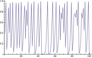
I was then asked how this works. The idea is actually quite simple and well known. A time series generated from a map, such as the logistic map, or from a set of ODEs, such as the chaotic Rössler system, can show very different types of behaviour. For some parameter values they might behave rather regular and for others they might exhibit a quite complex type of behaviour. Let's consider the logistic map first.
ListLinePlot[NestList[4*#*(1 - #) &, RandomReal[], 100]]
The resulting time series looks like this:
When we change the paramter (in the example above "4") we obtain the well known bifurcation diagram.
M = 400; listlogistic =
Table[{\[Mu], NestList[\[Mu] *#*(1 - #) &, RandomReal[],M]}, {\[Mu], 3, 4, 0.0001}]; allcoords = Flatten[Table[Table[{listlogistic[[i, 1]], listlogistic[[i, 2, j]]}, {j, 380, M}], {i, 1, Length[listlogistic]}], 1]; ListPlot[allcoords, PlotStyle -> {Black, AbsolutePointSize[0.01]}, ImageSize -> 750]
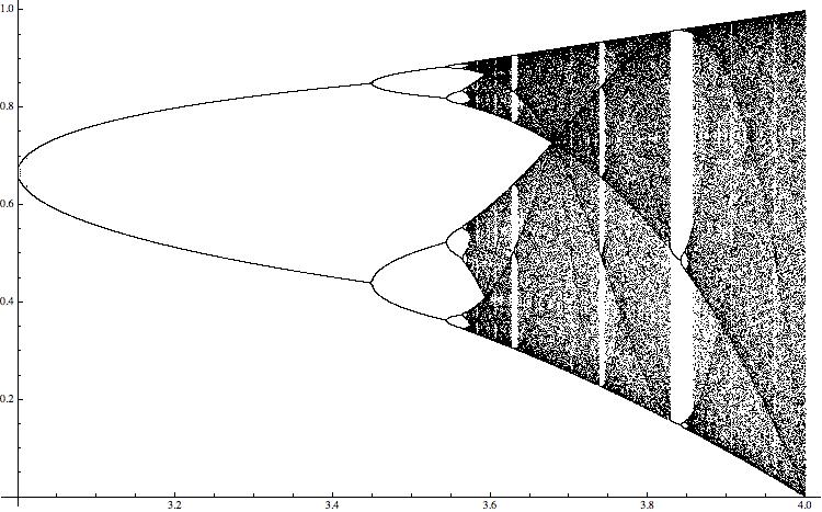
For different values of the paramter \ it shows the range of values of the resulting time series. The "black bands" indicate chaotic behaviour. A rather standard way to quantify this type of behaviour is the so-called Lyapunov exponent, which can be calculated easily in this case for all values of the paramter. (This will be more complicated in the higher dimensional example I will discuss later.)
(*Initiate*)
list5 = {};
(*Loop*)
For[a = 3.0, a <= 4, a = a + (4 - 1.5)/5000,
(*Generate data*)
data = NestList[a*#*(1 - #) &, RandomReal[], 10000];
smpl = 2000;
(*Evaluate Log[D[a*#*(1 - #) ,#]] at every point of the trajectory, sum up and add result to list*)
AppendTo[list5, {a, Total[Table[Log[Abs[a - 2.*a*data[[i]]]], {i, Length[data] - smpl, Length[data]}]]/smpl}]];
(*Plot*)
ListLinePlot[list5, ImageSize -> 750]
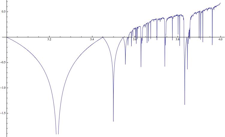
Positive values indicate chaotic behaviour; this corresponds to the black bands in the bifucation diagram. In higher dimensions it is more complicated to compute the Lyapunov exponent, particularly if we do not know the equations, but only have a time series. The following simple idea can help us to qualitatively assess the "complexity" of the time series. We first save the time series in a binary file, and determine its size - say in Bytes. We then compress the file using gzip, and again determine the size of the compressed file. The ratio of the two numbers, i.e. the compression rate, has information about the complexity of the time series. The code is very simple.
(*Initiate*)
list0 = {};
(*Change Paramter from 3 to 4 in 5000 steps *)
For[a = 3.0, a <= 4, a = a + (4. - 3.)/5000,
(*Generate data for paramter a*)
data = NestList[a*#*(1 - #) &, RandomReal[], 15000];
(*Write data to binary file*)
BinaryWrite["/Users/thiel/Desktop/sample.dat", data[[10000 ;;]],"Real32"]; Close["/Users/thiel/Desktop/sample.dat"];
(*Determine length of file*)
fsizebefore = FileByteCount["~/Desktop/sample.dat"];
(*gzip the file and determine new length*)
Run["gzip ~/Desktop/sample.dat"];
fsizeafter = FileByteCount["~/Desktop/sample.dat.gz"];
(*Clean up*)
Run["rm ~/Desktop/sample.dat.gz"]; Run["rm ~/Desktop/sample.dat"];
(*Collect data*)
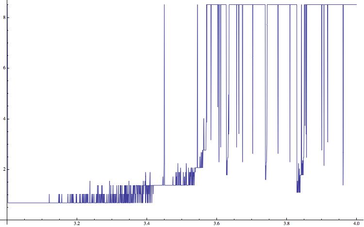
AppendTo[list0, {a, N[fsizeafter/fsizebefore]}]]; ListLinePlot[list0,ImageSize -> 750]
This gives the following figure:
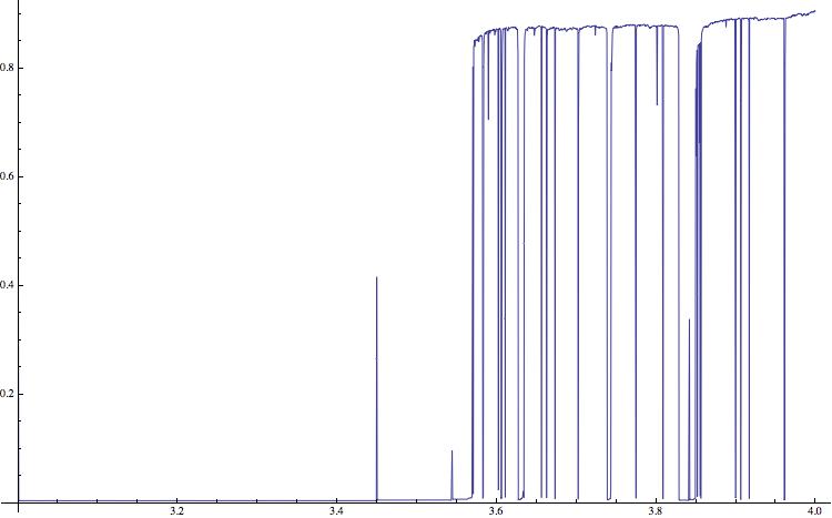
(Note that I am using a Mac and terminal commands. This will have to modified on a Windows machine.)
The compression rate can obviously not be negative. Low values indicate regular time series (which correspond to negative Lyapunov exponents in the figure above) and positive values indicate complex, potentially chaotic behaviour. The horizontal lines clearly indicate the periodic windows in the bifurcation diagram. The qualitative structure is very similar to the one of the diagram of the Lyaponov exponents. There are also peaks at the bifurcation points, e.g. at \=3; these are due to long transients at these points. In the literature it is claimed that the "gzip-entropy" is an estimate of the so-called algorithmic complexity.
I have tried out to get rid of the requirement to write the files to the hard drive using native Mathematica commands. There are two alternative approaches and the resulting figures.
list2 = {}; For[a = 3.0, a <= 4, a = a + (4 - 1.5)/5000, data = NestList[a*#*(1 - #) &, RandomReal[], 15000]; AppendTo[list2, {a, Entropy[data[[10000 ;;]]]}]]; ListLinePlot[list2,ImageSize -> 750]
and
Monitor[list4 = {}; For[a = 3.0, a <= 4, a = a + (4 - 1.5)/5000, data = NestList[a*#*(1 - #) &, RandomReal[], 15000];
AppendTo[list4, {a, N[ByteCount[Compress[Flatten[RealDigits[data[[10000 ;;]]]]]]/ByteCount[Flatten[RealDigits[data[[10000 ;;]]]]]]}]], a]; ListLinePlot[list4, ImageSize -> 750]
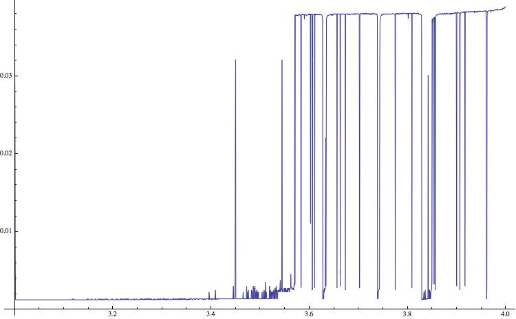
It appears that the two approaches that use Mathematica functions and do not rely on the external "gzip" give reasonable results as well. I am using solid state drives, so the speed up is not very large.
One might wonder, why we do not directly estimate the Lyapunov exponents, which can be done using e.g. Wolf's algorithm:
http://nzaier.com/nzaierbb/system/upload_files/Physica1985_wolf_LyapunovExpo.pdfThe point is that the gzip method is very easy to implement and rather fast. Let's consider the chaotic Roessler system.
(*Integrate*)
sols = NDSolve[
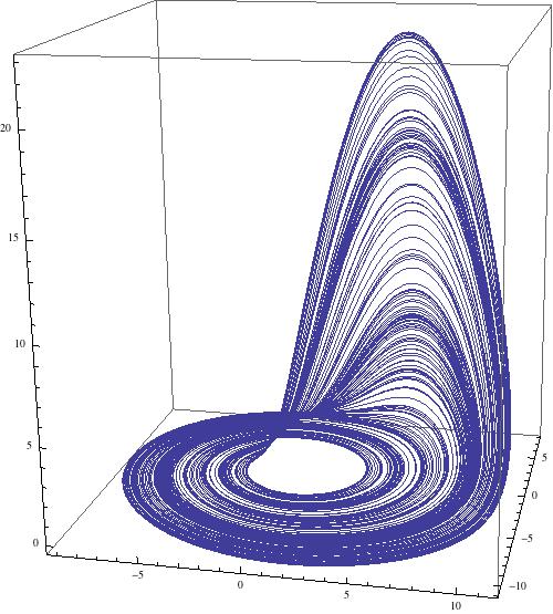
{D[x[t], t] == -y[t] - z[t], D[y[t], t] == x[t] + a y[t], D[z[t], t] == b + (x[t] - c) z[t], x[0] == RandomReal[], y[0] == RandomReal[], z[0] == RandomReal[]} /. {a -> 0.2, b -> 0.2, c -> 5.7}, {x, y, z}, {t, 0, 3000}, MaxSteps -> Infinity];
(*Plot; do not show transient, i.e. start at t=2000*)
ParametricPlot3D[{x[t], y[t], z[t]} /. sols, {t, 2000, 3000}, PlotRange -> All, ImageSize -> 500, PlotPoints -> 1000]
which gives
Let's sweep the paramter space from where a=b range from 0.2 to 0.3 and c goes from 20 to 45. The following command runs for slightly less then 6300 seconds on my laptop.
AbsoluteTiming[Monitor[listros = {};
(*Set up the loops for the paramter sweep, use 100 steps for a and for c *)
For[c = 20.0, c <= 45.0, c = c + (45. - 20.)/100.,
For[a = 0.2, a <= 0.3, a = a + (0.3 - 0.2)/100.,
(*Integrate the ODEs*)
sols = NDSolve[{D[x[t], t] == -y[t] - z[t], D[y[t], t] == x[t] + a y[t], D[z[t], t] == b + (x[t] - c) z[t], x[0] == RandomReal[], y[0] == RandomReal[], z[0] == RandomReal[]} /. b -> a, {x, y,z}, {t, 0, 2000}, MaxSteps -> Infinity];
(*Sample the time series, discard transient of 100 points*)
data = Table[{t, Part[x[t] /. sols, 1]}, {t, 1000, 2000, 0.2}];
(*Write the data to binary file*)
BinaryWrite["/Users/thiel/Desktop/sample.dat", data[[2000 ;;]],"Real64"]; Close["/Users/thiel/Desktop/sample.dat"];
(*Determine file size*)
fsizebefore = FileByteCount["~/Desktop/sample.dat"];
(*Compress and determine new file size*)
Run["gzip ~/Desktop/sample.dat"];
fsizeafter = FileByteCount["~/Desktop/sample.dat.gz"];
(*Clean up*)
Run["rm ~/Desktop/sample.dat.gz"];
Run["rm ~/Desktop/sample.dat"];
(*Collect results*)
AppendTo[listros, {c, a, N[fsizeafter/fsizebefore]}]]], {c, a}];]
Note that I only use the x-component of the system. The result can be plotted using
ListDensityPlot[listros, InterpolationOrder -> 0, ColorFunction -> "Rainbow", PlotRange -> All, PlotLegends -> Placed[Automatic, Right]]
which gives
The structures do not become very clear, but after a bit of "creative (and clumsy) rescaling"
listrosnorm = (listros[[All, 3]] - Min[listros[[All, 3]]])/(Max[listros[[All, 3]]] - Min[listros[[All, 3]]]);
listrosnorm2 = (listrosnorm - Mean[listrosnorm])/StandardDeviation[listrosnorm];
listnorm = Table[{listros[[k, 1]], listros[[k, 2]], Exp[listrosnorm2[[k]]]}, {k,1, Length[listrosnorm]}]
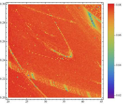
they become much clearer:
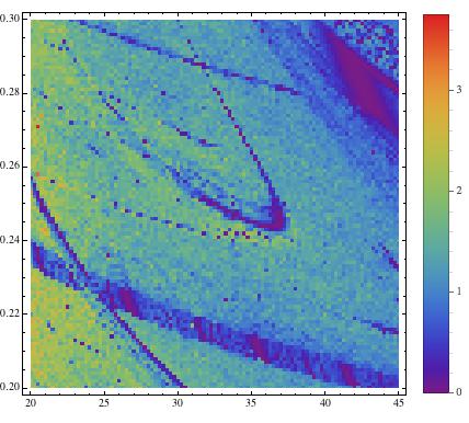
The blue regions indicate regular, e.g. periodic behaviour, and the green/red regions mean irregular, e.g. chaotic. This method allows us to screen large ranges of paramters to better understand the behaviour of a system. Note that in the middle of the image we start recognising a periodic (blue) structure that is called "shrimp". The following image uses a more precise method (Recurrence Plots) to esimate the correlation entropy of the same paramter region.
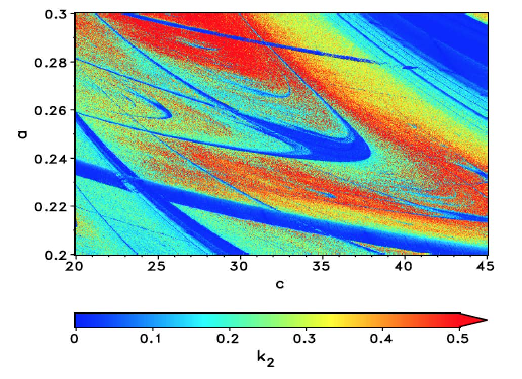
The periodic (blue) regions are much clearer now and the colours indicate how chaotic/erratic the system is, but that comes at the cost of CPU time. This figure was obtained using the computer cluster of my home institute. In this case the magnitude of the values that are colour-coded actually have meaning and are not only "proxies" as in the case of the gzip entropies above. I am currently optimising some Mathematica code and hope to be able to provide a piece of code soon, which will generate similar high quality pictures on a laptop. Mathematica's ability to use multiple CPUs, and other built in functions, such as curve-fitting, will be very useful to speed up the program.
There are several interesting features in this figure. First, there is the dominating "shrimp". Note that there are smaller shrimp below its "antennae". This shrimp structure is in fact fractal. A careful study of the figure allows us to guess what types of bifurcations occur and can provide useful information for a thorough bifurcation analysis.
None of the codes presented here is optimised at all. I just wanted to answer the question how to use gzip to estimate the behaviour of time series and how to screen larger regions of the paramter space. The method is quite quick and very dirty...


