The example differential equation is Troesch's equation, in which the following expression equals 0, with boundary conditions x(0) = 0 and x(1) = 1.
In[1]:= troesch = y''[x] - 5 Sinh[5 y[x]];
NDSolve is not able to solve this problem.
In[2]:= AbsoluteTiming[NDSolve[{troesch == 0, y[0] == 0, y[1] == 1}, y, x]]
During evaluation of In[2]:= NDSolve::ndsz: At x == 0.9555766885690343`, step size is effectively zero; singularity or stiff system suspected.
Out[2]= {0.194423,
NDSolve[{-5 Sinh[5 y[x]] + (y^\[Prime]\[Prime])[x] == 0, y[0] == 0,
y[1] == 1}, y, x]}
The following function generates the linearized expression.
The term noms refers to the corresponding variables
in the linearized expression.
In[3]:= lin[expr_, vars_, noms_] :=
Module[{r =
Thread[vars -> noms]}, (expr /.
r) + (vars - noms).((D[expr, #] & /@ vars) /. r)] // Simplify
lintroesch is the linearized differential equation. ys is the starting solution.
In[4]:= lintroesch[ys_] = lin[troesch, {y[x], y''[x]}, {ys[x], ys''[x]}]
Out[4]= -5 Sinh[5 ys[x]] + 25 Cosh[5 ys[x]] (-y[x] + ys[x]) + (y^\[Prime]\[Prime])[x]
iter calculates the improved solution, given the starting solution as input.
In[5]:= iter[ys_] :=
NDSolveValue[{lintroesch[ys] == 0, y[0] == 0, y[1] == 1}, y, {x, 0, 1},
InitialSeeding -> {y'[0] == ys'[0]}]
Using NestList, we generate a series of solutions,
each one based on the previous result.
The initial solution is simply a straight line
implementing the boundary conditions.
In[6]:= AbsoluteTiming[l = NestList[iter, # &, 7];]
Out[6]= {0.274403, Null}
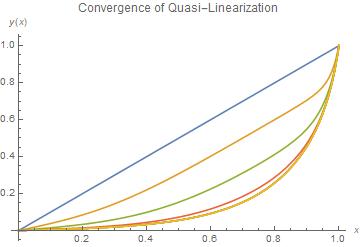
Plotting the results shows the convergence.
In[7]:= Plot[Evaluate[Through[l[x]]], {x, 0, 1}, AxesLabel -> {x, y[x]},
PlotLabel -> "Convergence of Quasi-Linearization" ]
The values converged value of the initial slope
can be used as an InitialSeeding for NDSolve
In[8]:= Table[l[[i]]'[0], {i, 8}]
Out[8]= {1, 0.366249, 0.142711, 0.0611296, 0.0461928, 0.0457509, 0.0457504, 0.0457504}
In[9]:= nsln = NDSolve[{troesch == 0, y[0] == 0, y[1] == 1}, y, x,
InitialSeeding -> {y'[0] == 0.046}];
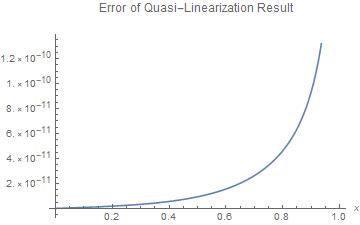
The result of the quasi-linearization is extremely close
to the result found by NDSolve with a good estimate of the starting slope.
In[10]:= Plot[l[[8]][x] - (y[x] /. nsln[[1]]), {x, 0, 1}, AxesLabel -> {x,},
PlotLabel -> "Error of Quasi-Linearization Result"]