Message Boards Message Boards

Solving Boundary Value ODEs With Quasi-Linearization

The example differential equation is Troesch's equation, in which the following expression equals 0, with boundary conditions x(0) = 0 and x(1) = 1.

In[1]:= troesch = y''[x] - 5 Sinh[5 y[x]];

 NDSolve is not able to solve this problem.

In[2]:= AbsoluteTiming[NDSolve[{troesch == 0, y[0] == 0, y[1] == 1}, y, x]]

During evaluation of In[2]:= NDSolve::ndsz: At x == 0.9555766885690343`, step size is effectively zero; singularity or stiff system suspected.

Out[2]= {0.194423, 
 NDSolve[{-5 Sinh[5 y[x]] + (y^\[Prime]\[Prime])[x] == 0, y[0] == 0, 
   y[1] == 1}, y, x]}

 The following function generates the linearized expression.  
The term noms refers to the corresponding variables 
in the linearized expression.

In[3]:= lin[expr_, vars_, noms_] := 
 Module[{r = 
     Thread[vars -> noms]}, (expr /. 
      r) + (vars - noms).((D[expr, #] & /@ vars) /. r)] // Simplify

 lintroesch is the linearized differential equation.  ys is the starting solution.

In[4]:= lintroesch[ys_] = lin[troesch, {y[x], y''[x]}, {ys[x], ys''[x]}]

Out[4]= -5 Sinh[5 ys[x]] + 25 Cosh[5 ys[x]] (-y[x] + ys[x]) + (y^\[Prime]\[Prime])[x]

 iter calculates the improved solution, given the starting solution as input.

In[5]:= iter[ys_] :=  
 NDSolveValue[{lintroesch[ys] == 0, y[0] == 0, y[1] == 1}, y, {x, 0, 1}, 
  InitialSeeding -> {y'[0] == ys'[0]}]

Using NestList, we generate a series of solutions, 
each one based on the previous result.  
The initial solution is simply a straight line 
implementing the boundary conditions.

In[6]:= AbsoluteTiming[l = NestList[iter, # &, 7];]

Out[6]= {0.274403, Null}

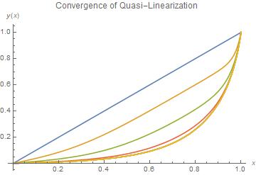
 Plotting the results shows the convergence.

In[7]:= Plot[Evaluate[Through[l[x]]], {x, 0, 1}, AxesLabel -> {x, y[x]}, 
 PlotLabel -> "Convergence of Quasi-Linearization" ]
enter image description here

 The values converged value of the initial slope 
can be used as an InitialSeeding for NDSolve

In[8]:= Table[l[[i]]'[0], {i, 8}]

Out[8]= {1, 0.366249, 0.142711, 0.0611296, 0.0461928, 0.0457509, 0.0457504, 0.0457504}

In[9]:= nsln = NDSolve[{troesch == 0, y[0] == 0, y[1] == 1}, y, x, 
  InitialSeeding -> {y'[0] == 0.046}];


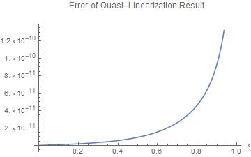
The result of the quasi-linearization is extremely close 
to the result found by NDSolve with a good estimate of the starting slope.

In[10]:= Plot[l[[8]][x] - (y[x] /. nsln[[1]]), {x, 0, 1}, AxesLabel -> {x,}, 
 PlotLabel -> "Error of Quasi-Linearization Result"]
enter image description here

POSTED BY: Frank Kampas
5 Replies

the solutions are slightly different

In[17]:= AbsoluteTiming[
 sol = NDSolve[{y''[x] - 5*Sinh[5*y[x]] == 0, y[0] == 0, y[1] == 1}, 
    y, {x, 0, 1}, Method -> "ExplicitEuler", 
    "StartingStepSize" -> 1/100];]

Out[17]= {0.0407043, Null}

In[19]:= y'[0] /. sol

Out[19]= {0.0538005}

In[22]:= x'[0] /. nsln

Out[22]= {0.0457504}

In[23]:= Plot[(x[t] /. nsln) - (y[t] /. sol), {t, 0, 1}]

enter image description here

It might be better to use the ExplicitEuler result to set an InitialSeeding for the default method.

POSTED BY: Frank Kampas

With this code works fine:

sol = NDSolve[{y''[x] - 5*Sinh[5*y[x]] == 0, y[0] == 0, y[1] == 1}, y, {x, 0, 1}, Method -> "ExplicitEuler", 
"StartingStepSize" -> 1/100];
Plot[y[x] /. sol, {x, 0, 1}, PlotRange -> All]

Regards M.I.

POSTED BY: Mariusz Iwaniuk
 Another approach to finding an InitialSeeding for Troesch's equation
is the Principle of Least Action, by considering the equation to be an 
equation of motion. 

 A Lagrangian can be constructed with its equation of motion being
Troesch's equation.

In[1]:= Needs["VariationalMethods`"]

In[2]:= EulerEquations[1/2 x'[t]^2 + Cosh[5 x[t]], x[t], t]

Out[2]= 5 Sinh[5 x[t]] - (x^\[Prime]\[Prime])[t] == 0

 The solution to the boundary value equation of motion can be constructed
 by minimizing the Action, which is the integral of the Lagrangian
  over the time period.  The Lagrangian is the kinetic energy minus
  the potential energy.  The two terms can be discretized, using a finite
  difference approximation for the time derivative.

 Discretized variables with bounds:

In[3]:= vwb = Table[{x[t], -1, 2}, {t, 0, 1, 1/20}];

Discretized approximation to integral of kinetic energy 

In[4]:= sumKE = 1/20*1/
    2 Sum[((x[t + 1/40] - x[t - 1/40])/(1/20))^2, {t, 1/40, 39/40, 1/20}] // 
   Expand;

 Discretized approximation to the integral of the potential energy

In[5]:= sumPE = - (1/21) Sum[Cosh[5 x[t]], {t, 0, 1, 1/20}];

 Minimize the discretized approximation to the Action

In[6]:= AbsoluteTiming[nmsln = NMinimize[{sumKE - sumPE, x[0] == 0, x[1] == 1}, vwb];]

Out[6]= {0.123725, Null}

 Construct an interpolation function from the solution

In[7]:= int = Interpolation[Table[{t, x[t]}, {t, 0, 1, 1/20}] /. nmsln[[2]]];

 Find the derivative at t = 0

In[8]:= int'[0]

Out[8]= 0.0523738

 Use the derivative as an Initial Seeding

In[9]:= AbsoluteTiming[
  nsln = NDSolve[{5 Sinh[5 x[t]] - (x^\[Prime]\[Prime])[t] == 0, x[0] == 0, 
     x[1] == 1}, x, t, InitialSeeding -> {x'[0] == 0.0523}]];

 Plot the result

enter image description here

POSTED BY: Frank Kampas

Thanks for pointing out the article.

POSTED BY: Frank Kampas
Anonymous User
Anonymous User
Posted 5 years ago

Troesch’s equation is a boundary value problem (BVP) expressed as where prime denotes differentiation with respect to x and n (sinh(n y)) is known as Troesch’s parameter.

https://www.hindawi.com/journals/mpe/2012/208375/ a comparison of convergence speed of the various solutions

POSTED BY: Anonymous User
Reply to this discussion
Community posts can be styled and formatted using the Markdown syntax.
Reply Preview
Attachments
Remove
or Discard

Group Abstract Group Abstract