First a suggestion: you might use NDSolve instead of DSolve.
To follow up on Sean Clarke's comment, here is a way to replace Real numbers by symbolic coefficients. One issue is that two of the numbers are very close. They agree up to 40 digits, but I left them as different coefficients, even though it might slow down DSolve a little.
(* store IVP in a variable *)
ivp = {-0.0533997864008543965824134994660021359914560341760000000000009213431`49.52287874528033 v1''[t] +
0.1333909976860092559629760311498754004983980064080000000000023688355`49.52287874528033 v1[t] == -0.283018867924528301886792 +
0.005014252567755304845165779349483873526333219876 E^(-2.81465156744174009869712731637825723649652499385228694169 t) +
0.008586511345122480854910534410479478741705706287 E^(-1.732050807568877293527446341505872366942805253810158290235 t) +
0.25001517408748706819836422234433174826 E^(-0.80570784117217514973733627569314947705823994352092046887 t) +
0.09989713599393614000262596240276808141 E^(0.80570784117217514973733627569314947705823994352092046887 t) -
0.028611431245442879573315596710230279738501719103 E^(1.732050807568877293527446341505872366942805253810158290235 t) -
0.002487972403539495602226406704527557128725712261`27.907709483032015 *
E^(2.81465156744174009869712731637825723649652499385228694169`40.50024606432001 t) +
0.24029903880384478462086074759700961196`27.907212282747974 t,
v1[0] == 0, v1[1] == 1};
numbers = Union[Cases[ivp, x_Real :> Abs[x], Infinity]] (* get the numerical coefficients *)
(*
Out[5]= {0.002487972403539495602226406705,
0.005014252567755304845165779349483873526333219876,
0.008586511345122480854910534410479478741705706287,
0.02861143124544287957331559671023027973850171910,
0.05339978640085439658241349946600213599145603417600,
0.09989713599393614000262596240276808141,
0.13339099768600925596297603114987540049839800640800,
0.2402990388038447846208607476,
0.25001517408748706819836422234433174826,
0.283018867924528301886792,
0.80570784117217514973733627569314947705823994352092046887,
1.732050807568877293527446341505872366942805253810158290235,
2.8146515674417400986971273163782572364965,
2.8146515674417400986971273163782572364965249938522869417}
*)
coeffRules = (* create replacement rules to replace number by coeff[n] *)
Thread /@ {#, Distribute[-#, Rule, Times]} &[numbers -> Array[coeff, Length@numbers]] // Flatten;
ivp /. coeffRules (* see if the rules work *)
(*
Out[8]= {coeff[7] v1[t] -
coeff[5] (v1^\[Prime]\[Prime])[t] == -E^(t coeff[13]) coeff[1] +
E^(-t coeff[14]) coeff[2] + E^(-t coeff[12]) coeff[3] -
E^(t coeff[12]) coeff[4] + E^(t coeff[11]) coeff[6] + t coeff[8] +
E^(-t coeff[11]) coeff[9] - coeff[10], v1[0] == 0, v1[1] == 1}
*)
solCoeff = DSolve[ivp /. coeffRules, {v1[t]}, t]; (* solve the symbolic IVP *)
Reverse /@ coeffRules[[;; Length@numbers]] (* show that reversing the rules creates the inverse substitution *)
(*
Out[10]= {coeff[1] -> 0.002487972403539495602226406705,
coeff[2] -> 0.005014252567755304845165779349483873526333219876,
coeff[3] -> 0.008586511345122480854910534410479478741705706287,
coeff[4] -> 0.02861143124544287957331559671023027973850171910,
coeff[5] -> 0.05339978640085439658241349946600213599145603417600,
coeff[6] -> 0.09989713599393614000262596240276808141,
coeff[7] -> 0.13339099768600925596297603114987540049839800640800,
coeff[8] -> 0.2402990388038447846208607476,
coeff[9] -> 0.25001517408748706819836422234433174826,
coeff[10] -> 0.283018867924528301886792,
coeff[11] -> 0.80570784117217514973733627569314947705823994352092046887,
coeff[12] -> 1.732050807568877293527446341505872366942805253810158290235,
coeff[13] -> 2.8146515674417400986971273163782572364965,
coeff[14] -> 2.8146515674417400986971273163782572364965249938522869417}
*)
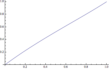
sol = solCoeff /. (Reverse /@ coeffRules[[;; Length@numbers]]); (* substitute the numbers for the coeff[n] *)
Plot[v1[t] /. First@sol, {t, 0, 1}]
Comparison with Ilian Gachevski's solution
There's no significant difference
solFSimp = DSolve[FullSimplify@ivp, {v1[t]}, t];
diffFSimp = Table[(v1[t] /. First@sol) - (v1[t] /. First@solFSimp), {t, 0, 1, 1/50000}];
{Min[diffFSimp], Max[diffFSimp]}
(*
Out[34]= {0.*10^-13, 0.*10^-12}
*)
Comparison with NDSolve
We'll construct two solution, a machine-precision one nsol and a one that takes advantage of the high-precision coefficients. The machine-precision solution is calculated very fast, and the higher precision solution is slower but takes only a fraction of a second.
nsol = NDSolve[ivp, {v1[t]}, {t, 0, 1}];
Min[Precision /@ numbers] (* find the min. precision of the coefficients *)
(*
Out[20]=
23.4518
*)
nsolprec = NDSolve[ivp, {v1[t]}, {t, 0, 1},
PrecisionGoal -> Min[Precision /@ numbers] - 3, (* need some slop in the goals *)
AccuracyGoal -> Min[Precision /@ numbers] - 1,
WorkingPrecision -> Min[Precision /@ numbers]];
The default AccuracyGoal and PrecisionGoal are one-half of MachinePrecision, or about 10^-8:
Plot[Evaluate[(v1[t] /. First@sol) - (v1[t] /. First@nsol)], {t, 0, 1}, PlotRange -> All]
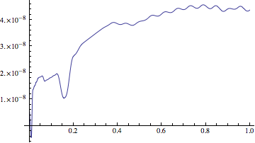
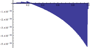
AccuracyGoal and PrecisionGoal are not always achievable, but they make the solution agree much better with the symbolic solution:
diffPrec = Table[(v1[t] /. First@sol) - (v1[t] /. First@nsolprec), {t, 0, 1, 1/50000}];
{Min[diffPrec], Max[diffPrec]}
(*
Out[38]= {-5.3365*10^-16, 2.117*10^-17}
*)
ListPlot[diffPrec, DataRange -> {0, 1}, PlotRange -> All]