MODERATOR NOTE: a submission to computations art contest, see more: https://wolfr.am/CompArt-22
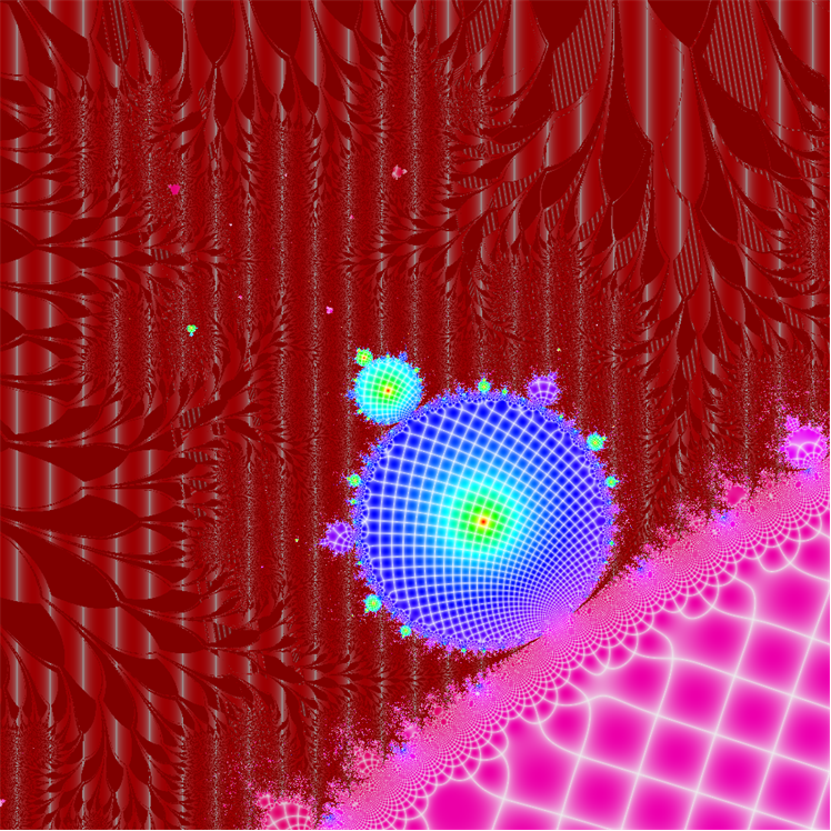
Showing Abs and Arg fields of Mandelbrot set under 200 iterations
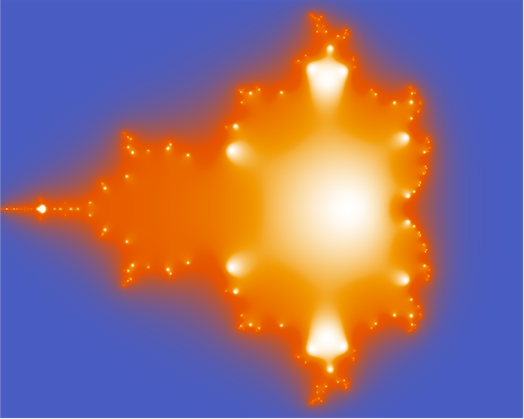
Showing Abs field of Mandelbrot set under 9 iterations
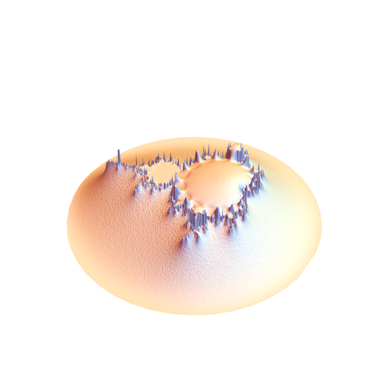
Showing Re vs. Im complex mapping of Mandelbrot set under 200 iterations
Mandelbrot Set on Neural Network
The MXNet-based neural network framework has been introduced to Wolfram Language since version 11. It is mostly designed for deep learning. However if we think about it, neural network is merely another fancy way to implement a certain program. As more and more functions are supported, it is now possible for us to "compile" general numerical program to neural network, which essentially gives us an interface to GPGPU parallel ability without the hassle of low-level coding.
Inspired by Brian's recent post on MathCompile, we demonstrate in this post how to implement a neural network to compute the Mandelbrot set.
Utilities
As usual here is the code dump of some helper functions. Readers can evaluate then safely skip this section.
code dump of helper functions
ClearAll[pipe, branch]
pipe   = RightComposition;
branch = Through@*{##} &;
Needs["NeuralNetworks`"]
Clear[netInputPortSort]
netInputPortSort[inPortLst_List] := Function[origNet, netInputPortSort[origNet, inPortLst]]
netInputPortSort[origNet_NetGraph, inPortLst_List] :=
 Block[{NetGraph = Inactive[NetGraph], fullnet, net},
           fullnet         = origNet
           ; net           = fullnet[[1]]
           ; net["Inputs"] = AssociationThread[Rule[inPortLst, inPortLst /. net["Inputs"]]]
           ; ReplacePart[fullnet, 1 -> net]
      ] // Activate
Basic concept
The center of the Mandelbrot set computation is a simple iteration:
$$\left\{ \begin{align} z_n &= c+z_{n-1}^2 \\ z_0 &= 0 \end{align} \right.$$
Under simple iteration it leads to the Mandelbrot set.
Block[{region, c, faclets}
         ,
         (* random-points as different c for iteration: *)
         region = Disk[{-.5, 0}, 2] // DiscretizeGraphics // DiscretizeRegion[#, MaxCellMeasure -> .0001] &
         ; faclets = MeshCells[region, 2][[;; , 1]]
         ; c = MeshCoordinates[region].{1, I}
         ;(* The iteration taking place simultaneously for all c, nested 21 steps: *)
         Nest[Function[z, z^2 + c], 0, 21] //
              (* Visualizing the result: *)
              pipe[
                      pipe[(* Regularizing the norm for a clear visualization: *)
                           Abs, HistogramTransform, Rescale, (1 - #)^2 &]
                      , Append[ReIm[c]\[Transpose], #]\[Transpose] &
                      , Graphics3D[
                                    GraphicsComplex[#, {EdgeForm[], Polygon@faclets}]
                                    , Boxed -> False, SphericalRegion -> True, RotationAction -> "Fit"
                                    , ViewPoint -> {1, -2.4, 2.4}, ViewVertical -> {0, 0, 1}
                                  ] &
                  ]
     ]
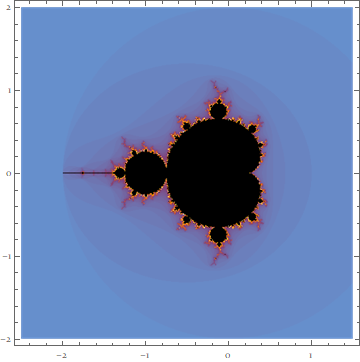
Using the built-in MandelbrotSetPlot function, it's straightforward to plot the traditional Mandelbrot set visualization:
MandelbrotSetPlot[{-2.5 - 2 I, 1.5 + 2 I}]
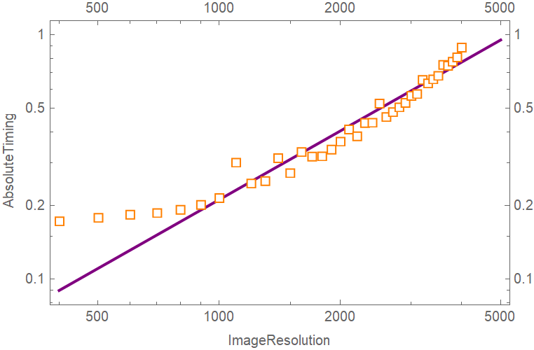
With some test we can notice that, for fixed MaxIterations, the relationship between computing time of MandelbrotSetPlot and ImageResolution follows a power law.
builtInTimeTest = {#, AbsoluteTiming[MandelbrotSetPlot[{-2.5 - 2 I, 1.5 + 2 I}, MaxIterations -> 100, ImageResolution -> #];][[1]]} & /@ Range[101, 4001, 100]

NonlinearModelFit[builtInTimeTest, a r^k, {a, k}, r][r] //
  LogLogPlot[#, {r, 400, 5000}, PlotStyle -> Directive[Red, AbsoluteThickness[2]], Frame -> True, FrameTicks -> All] & //
  Show[{#
        , ListLogLogPlot[builtInTimeTest, PlotMarkers -> "OpenMarkers", PlotRange -> All]
        }, FrameLabel -> {"ImageResolution", "AbsoluteTiming"}] &
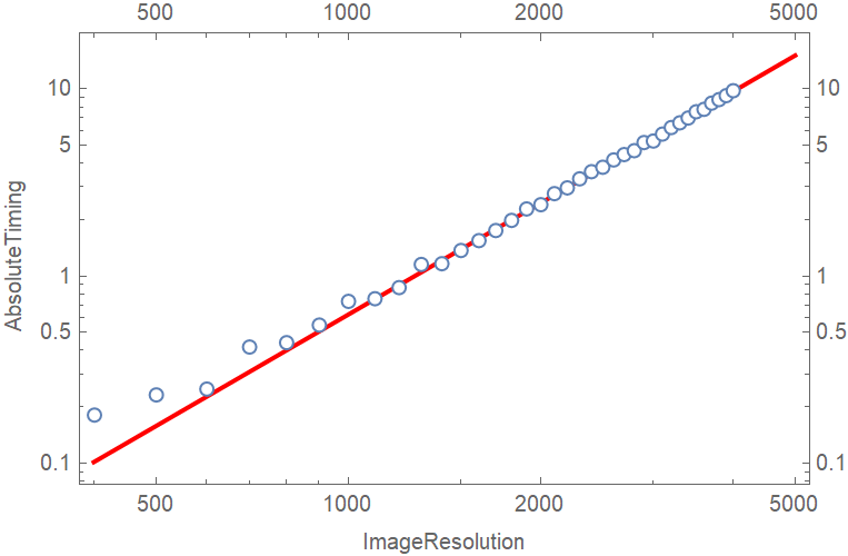
This is a scenario where parallel computation might make a difference.
Mandelbrot set on neural network -- A naïve attempt
The implementation
Iteration core net
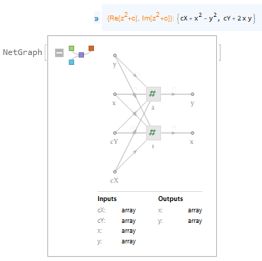
Neural network (short for NN) doesn't support complex number (yet). Aside from that, the iteration formula is simple enough for ThreadingLayer:
iterNet = Module[{c = cX + cY I, z = x + y I},
  z^2 + c // pipe[
                    ReIm, ComplexExpand, Echo[#, "{Re[\!\(\*SuperscriptBox[\(z\), \(2\)]\)+c], Im[\!\(\*SuperscriptBox[\(z\), \(2\)]\)+c]}:"] &
                    , Map@pipe[
                                 Inactive[Function][{cX, cY, x, y}, #] &
                                 , Activate
                                 , ThreadingLayer
                              ]
                    , Inactive[NetGraph][#
                                            , {
                                                   (NetPort /@ StringSplit["cX,cY,x,y", ","]) -> # & /@ {1, 2}
                                                   , 1 -> NetPort["x"], 2 -> NetPort["y"]
                                              }
                                        ] &
                    , Activate
                 ]
  ]
It's very easy to perform the iteration with the help of Nest / NestList.
Block[{region, c, xyInit, result}
         ,
         (* random-points as different c for iteration: *)
         region = Disk[{0, 0}, .5] // DiscretizeGraphics // DiscretizeRegion[#, MaxCellMeasure -> .01] &
         ; c = MeshCoordinates[region].{1, I} // ReIm
         ; c = AssociationThread[StringSplit["cX,cY", ","], c\[Transpose]]
         ; xyInit = AssociationThread[StringSplit["x,y", ","], 0*Values[c]]
         ; result = NestList[
                                pipe[
                                      Map[Clip[#, {-2, 2}] &]
                                      , Join[c, #] &
                                      , iterNet
                                    ]
                                , xyInit, 20
                            ]
         ; result //
             pipe[
                     Values, Rest, Map@Transpose
                     , Transpose
                     , MapThread[{#2, BSplineCurve@#1} &, {#, # // Length // Range // N // Rescale // Map[ColorData["Rainbow"]]}] &
                     , Graphics[#, Frame -> True, FrameTicks -> All, PlotRange -> {GoldenRatio {-1, 1}, {-1, 1}}, PlotRangeClipping -> True] &
                 ]
     ]
Nest net
Now we have the core net representing the iteration formula, we need to mimic the functionality of Nest[f, expr, n] fully on a neural network.
The go-to function is of course NetNestOperator. However in our case, the same $c$ is used repeatedly for all iterations, so we'd like to pass it directly to each iteration. Thus, we do it with the following customized NetNestPartialOperator function:
ClearAll[NetNestPartialOperator]
NetNestPartialOperator[net_, staticPorts_List, nestPort_, iterNum_Integer] :=
 Module[{pIdx, netIdx, staticpath, nestpath},
  netIdx = Range[iterNum]
  ; pIdx = AssociationThread[staticPorts, staticPorts // Length // Range // Map[ToString]]
  ; staticpath = Function[p, NetPort["static" <> pIdx[p]] -> (NetPort[#, p] & /@ netIdx)] /@ staticPorts
  ; nestpath = Thread[Flatten[{NetPort["nest"], netIdx // Most}] -> (NetPort[#, nestPort] & /@ netIdx)]
  ; Inactive[NetGraph][ConstantArray[net, iterNum], {staticpath, nestpath} // Flatten] //
       Activate //
       netInputPortSort[Flatten[{"nest", "static" <> # & /@ Values[pIdx]}]]
  ]
Basically our NetNestPartialOperator takes a net_NetGraph as the 1st argument. One of net's input ports, i.e. nestPort, is going to be nested across iterations; other input ports (i.e. staticPorts) will be feed in constant/non-nested values.
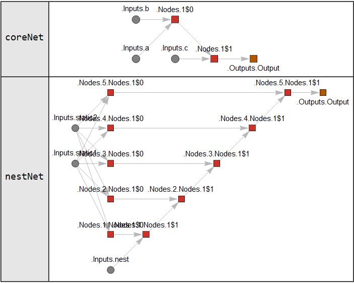
Here is a simple example realizing a 5 steps nest iteration Nest[Function[c,a+b+c],c0,5]:
Module[{coreNet, nestNet}
           , coreNet = NetGraph[{ThreadingLayer[#1+#2+#3&]}, {{NetPort["a"],NetPort["b"],NetPort["c"]}->1},"a"->"Real","b"->"Real","c"->"Real"]
           ; nestNet = NetNestPartialOperator[coreNet, {"a", "b"}, "c", 5]
           ; {
               {"coreNet", "nestNet"}
               , Quiet[
                         NetInformation[#, "MXNetNodeGraph"] // Graph[#, VertexSize -> 0.2, VertexLabels -> "Name"] &
                      ] & /@ {coreNet, nestNet}
             }\[Transpose] //
             Grid[#, Background -> {{GrayLevel[.9], None}, None}, Frame -> All, FrameStyle -> Black] &
      ]
The Mandelbrot net
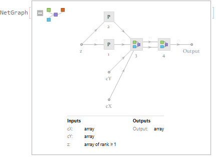
In order to construct a net suitable for NetNestPartialOperator, we merge the real and imaginary ports in iterNet into a single "complex" port.
zNet = NetGraph[{ReplicateLayer[1], ReplicateLayer[1], CatenateLayer[]}, {NetPort["1"] -> 1, NetPort["2"] -> 2, {1, 2} -> 3}];

nestcoreNet = NetGraph[
                        {PartLayer[1], PartLayer[2], iterNet, zNet}
                        , {
                               (NetPort[#] -> NetPort[3, #]) & /@ StringSplit["cX,cY", ","]
                             , NetPort["z"] -> {1, 2}
                             , {{1, 2}, StringSplit["x,y", ","]} // MapThread[(#1 -> NetPort[3, #2]) &]
                             , {StringSplit["x,y", ","], StringSplit["1,2", ","]} // MapThread[(NetPort[3, #1] -> NetPort[4, #2]) &]
                          }
                      ]
Thus a full net computing the Mandelbrot set is constructed as follows:
ClearAll[mandelbrot]
mandelbrot[iterNum_Integer?Positive] :=
     NetGraph[{
                  zNet
                , ElementwiseLayer[0 # &]
                , NetNestPartialOperator[nestcoreNet, StringSplit["cX,cY", ","], "z", iterNum]
              }, {
                  {NetPort["cX"], NetPort["cY"]} -> 1 -> 2
                , {2, NetPort["cX"], NetPort["cY"]} -> 3
              }
             ]
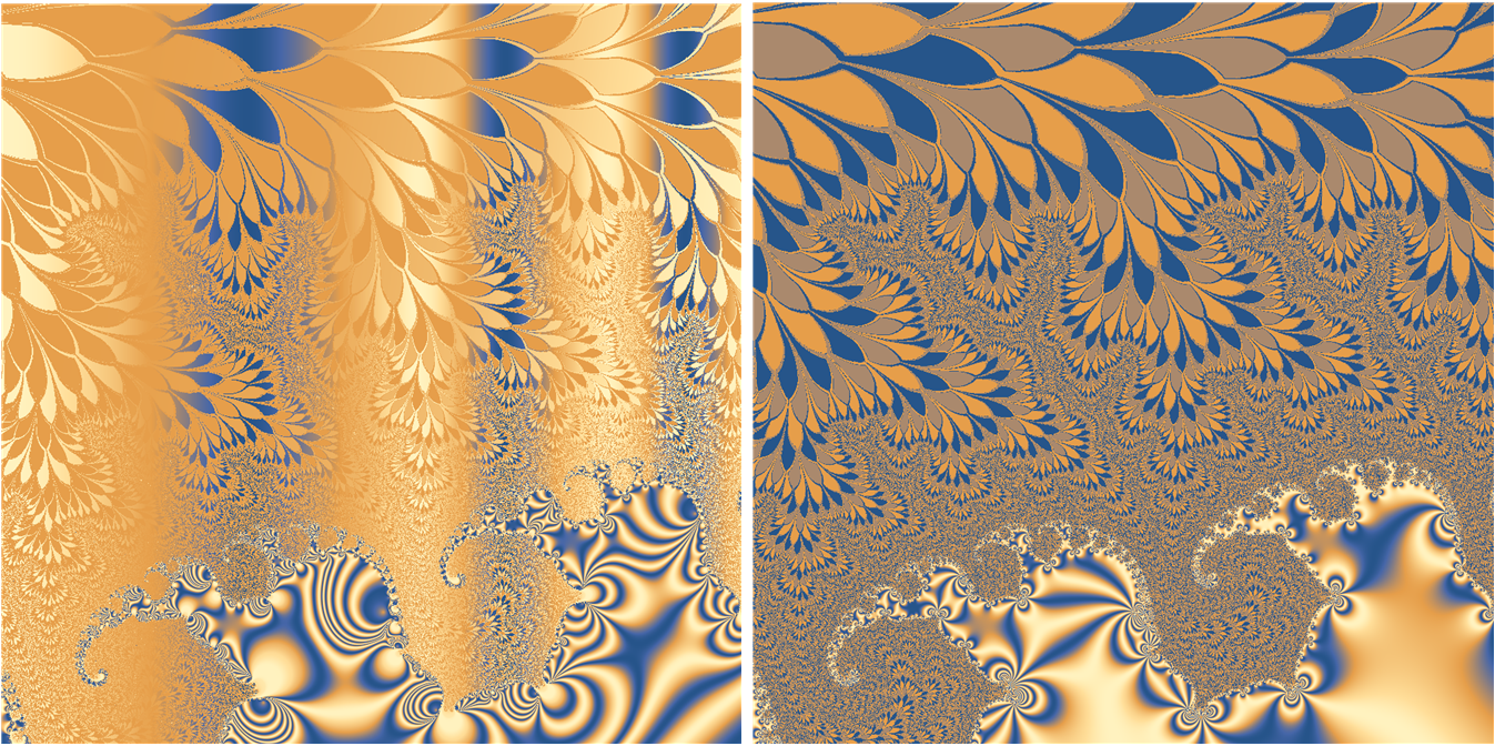
Results
We showcase our mandelbrot net with 9 iteration steps over the complex region ${-2-1.2I,1+1.2I}$, with a image resolution $401 \times 501$. The network is executed on a GPU (NVIDIA GeForce GTX 1050 Ti) with "Real64" precision.
mandelbrotF = mandelbrot[9];
result =
  Module[{region = {-2 - 1.2 I, 1 + 1.2 I}, resol = 501, aspr},
         region = region // ReIm // Transpose
         ; aspr = region.{-1, 1} // Reverse // Apply[Divide]
         ; resol = resol {1, aspr} // Round
         ; {resol, region} //
             pipe[
                   MapThread[Rescale[Range[#1] // N // Rescale, {0, 1}, #2] &]
                   , Tuples
                   , AssociationThread[{"cX", "cY"}, #\[Transpose]] &
                   , AbsoluteTiming[mandelbrotF[#, WorkingPrecision -> "Real64", TargetDevice -> "GPU"]] &
                   , pipe[
                            branch[pipe[First, Quantity[#, "Seconds"] &, Echo[#, "Computing time on NN:"] &], Last]
                            , Last]
                   , Developer`ToPackedArray
                   , ArrayReshape[#, {2, Sequence @@ resol}] &
                   , {1, I}.# &
                   , Transpose, Reverse
                 ]
        ];

(* Computing time on NN: 3.08505 s *)
result // Dimensions
(* {401, 501} *)
result //
   pipe[
         branch[
                 pipe[ Abs
                     , pipe[
                             branch[Flatten /* HistogramTransform, Dimensions /* Last]
                           , Apply@Partition
                           ]
                     , Rescale, (1 - #)^5 &
                     ]
               , pipe[Arg, Sin, Rescale]
               ]
       , Map @ pipe[
                     Image[#, ImageSize -> Length[#]] &
                   , Colorize[#, ColorFunction -> "DarkColorFractalGradient"] &
                   ]
       ]
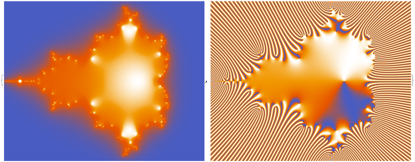
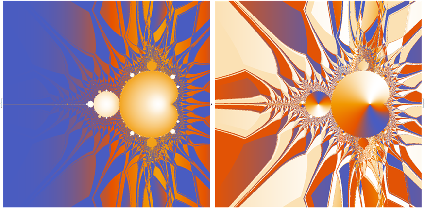
Note the highlighted periodic bulbs and Mandelbrot dendritic islands in the left image, and the pattern approximately following the external rays of the set in the right image.
As a comparison, here is the result from the same region, iteration steps and resolution using the built-in MandelbrotSetPlot function.
AbsoluteTiming[
                MandelbrotSetPlot[{-2 - 1.2 I, 1 + 1.2 I}, MaxIterations -> 9, ImageResolution -> 501]
              ] //
     pipe[
           branch[pipe[First, Quantity[#, "Seconds"] &, Echo[#, "Computing time:"] &], Last], Last
         , #[[1, 1]] &, Reverse, Image[#, ImageSize -> Dimensions[#][[1]]] &
         ]

(* Computing time: 0.187943 s *)
Clearly at this resolution scale, MandelbrotSetPlot is much faster than our neural-net function. But at a much larger resolution our function will eventually win.
myMandelbrotSetPlotTiming[resolution_Integer] :=
Module[ {region = {-2 - 1.2 I, 1 + 1.2 I}, aspr, resol}
, region = region // ReIm // Transpose
; aspr = region.{-1, 1} // Reverse // Apply[Divide]
; resol = resolution {1, aspr} // Round
; {resol, region} //
pipe[
MapThread[Rescale[Range[#1] // N // Rescale, {0, 1}, #2] &]
, Tuples
, AssociationThread[{"cX", "cY"}, #\[Transpose]] &
, AbsoluteTiming[mandelbrotF[#, WorkingPrecision -> "Real64", TargetDevice -> "GPU"];][[1]] &
, {resolution, #} &
]
]
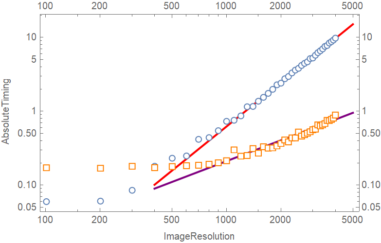
myTimeTest = myMandelbrotSetPlotTiming /@ Range[101, 4001, 100];
NonlinearModelFit[myTimeTest, a r^k, {a, k}, r][r] //
LogLogPlot[#, {r, 400, 5000}, PlotStyle -> Directive[Purple, AbsoluteThickness[2]], Frame -> True, FrameTicks -> All] & //
Show[ {
#
, ListLogLogPlot[myTimeTest, PlotMarkers -> Graphics[{FaceForm[White], EdgeForm[{Orange, AbsoluteThickness[1]}], Polygon[CirclePoints[4]]}, ImageSize -> 7], PlotRange -> All]
}
, FrameLabel -> {"ImageResolution", "AbsoluteTiming"}
] &
Comparing with previous benchmark result of MandelbrotSetPlot, we can see our NN-based function has an advantage when the image resolution is large enough.
Mandelbrot set on neural network -- Avoid overflow
Careful readers will find that for larger iteration steps and/or a larger computing region, our naïvely implemented mandelbrot will lead to overflow. That is of course due to the $c$ values leading to divergency. One simple way to avoid this overflow is to constrain the nested $z$ to a bounded region at every iteration step.
The implementation
A constrained iteration core net
The simplest way to constrain the nested $z$ is to clip it into a rectangle region.
iterNet = Module[{c = cX + cY I, z = x + y I},
  z^2 + c // pipe[
                   ReIm, ComplexExpand, Echo[#, "{Re[\!\(\*SuperscriptBox[\(z\), \(2\)]\)+c], Im[\!\(\*SuperscriptBox[\(z\), \(2\)]\)+c]}:"] &
                 , Map@pipe[
(* The constraint: -> *)     Block[{escR = 3}, escR Clip[#/escR]] &
                           , Inactive[Function][{cX, cY, x, y}, #] &
                           , Activate
                           , ThreadingLayer
                           ]
                 , Inactive[NetGraph][#
                                         , {
                                                (NetPort /@ StringSplit["cX,cY,x,y", ","]) -> # & /@ {1, 2}
                                                , 1 -> NetPort["x"], 2 -> NetPort["y"]
                                           }
                                     ] &
                 , Activate
                 ]
  ]
The Mandelbrot net
Re-evaluating the rest of the code leads to our simply constrained mandelbrotCons function.
nestcoreNet = NetGraph[
                        {PartLayer[1], PartLayer[2], iterNet, zNet}
                      , {
                          (NetPort[#] -> NetPort[3, #]) & /@ StringSplit["cX,cY", ","]
                        , NetPort["z"] -> {1, 2}
                        , {{1, 2}, StringSplit["x,y", ","]} // MapThread[(#1 -> NetPort[3, #2]) &]
                        , {StringSplit["x,y", ","], StringSplit["1,2", ","]} // MapThread[(NetPort[3, #1] -> NetPort[4, #2]) &]
                        }
                      ]
ClearAll[mandelbrotCons]
mandelbrotCons[iterNum_Integer?Positive] :=
     NetGraph[{
                zNet
              , ElementwiseLayer[0 # &]
              , NetNestPartialOperator[nestcoreNet, StringSplit["cX,cY", ","], "z", iterNum]
              },
              {
                {NetPort["cX"], NetPort["cY"]} -> 1 -> 2
              , {2, NetPort["cX"], NetPort["cY"]} -> 3
              }
             ]
Results
Now we can go for much larger iteration steps on a larger region.
mandelbrotConsF = mandelbrotCons[200];
result =
  Module[{region = {-3 - 2 I, 1 + 2 I}, resol = 1001, aspr},
         region = region // ReIm // Transpose
         ; aspr = region.{-1, 1} // Reverse // Apply[Divide]
         ; resol = resol {1, aspr} // Round
         ; {resol, region} //
             pipe[
                   MapThread[Rescale[Range[#1] // N // Rescale, {0, 1}, #2] &]
                   , Tuples
                   , AssociationThread[{"cX", "cY"}, #\[Transpose]] &
                   , AbsoluteTiming[mandelbrotConsF[#, WorkingPrecision -> "Real64", TargetDevice -> "GPU"]] &
                   , pipe[
                            branch[pipe[First, Quantity[#, "Seconds"] &, Echo[#, "Computing time on NN:"] &], Last]
                            , Last]
                   , Developer`ToPackedArray
                   , ArrayReshape[#, {2, Sequence @@ resol}] &
                   , {1, I}.# &
                   , Transpose, Reverse
                 ]
        ];

(* Computing time on NN: 6.29684 s *)
result // Dimensions
(* {1001, 1001} *)
result //
   pipe[
         branch[
                 pipe[ Abs
                     , pipe[
                             branch[Flatten /* HistogramTransform, Dimensions /* Last]
                           , Apply@Partition
                           ]
                     , Rescale, (1 - #)^5 &
                     ]
               , pipe[Arg, Sin, Rescale]
               ]
       , Map @ pipe[
                     Image[#, ImageSize -> Length[#]] &
                   , Colorize[#, ColorFunction -> "DarkColorFractalGradient"] &
                   ]
       ]
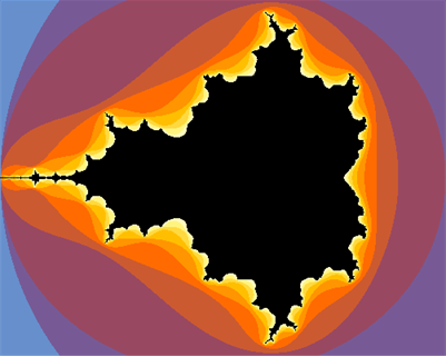
Or thresholding at 2 to get the classical Mandelbrot set.
result // Abs // UnitStep[2 - #] & // Image

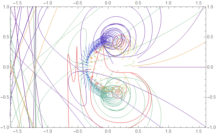
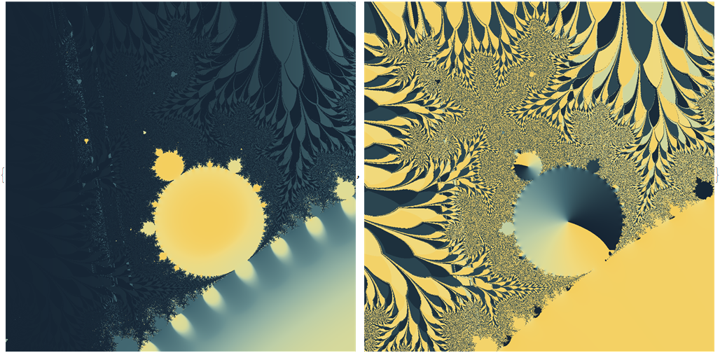
Zoom-in
For zoomed-in regions, this clipped version gives interesting results.
result =
  Module[{region = {-0.65 + 0.47 I, -0.4 + 0.72 I}, resol = 1001, aspr},
         region = region // ReIm // Transpose
         ; aspr = region.{-1, 1} // Reverse // Apply[Divide]
         ; resol = resol {1, aspr} // Round
         ; {resol, region} //
             pipe[
                   MapThread[Rescale[Range[#1] // N // Rescale, {0, 1}, #2] &]
                   , Tuples
                   , AssociationThread[{"cX", "cY"}, #\[Transpose]] &
                   , AbsoluteTiming[mandelbrotConsF[#, WorkingPrecision -> "Real64", TargetDevice -> "GPU"]] &
                   , pipe[
                            branch[pipe[First, Quantity[#, "Seconds"] &, Echo[#, "Computing time on NN:"] &], Last]
                            , Last]
                   , Developer`ToPackedArray
                   , ArrayReshape[#, {2, Sequence @@ resol}] &
                   , {1, I}.# &
                   , Transpose, Reverse
                 ]
        ];

(* Computing time on NN: 6.06289 s *)
result // pipe[
                branch[
                        pipe[ Abs
                            , pipe[branch[Flatten /* HistogramTransform, Dimensions /* Last], Apply@Partition]
                            , Rescale, (1 - #)^5 &, Sin[\[Pi]/2 #] &, Rescale
                            ]
                      , pipe[Arg, Sin[#/2] &, Rescale]
                      ]
              , Map@pipe[ Image[#, ImageSize -> Round[Length[#]/2]] &
                        , Colorize[#, ColorFunction -> "StarryNightColors"] &
                        ]
              ]
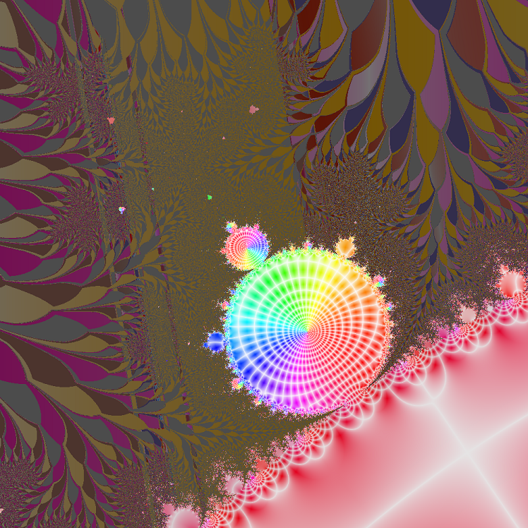
Complex map
We can also stylize the result any way we want, say, showing the complex mapping like the ComplexPlot.
Abs vs. Arg:
result // pipe[
                branch[
                        pipe[ Arg
                            , branch[
                                      pipe[Sin[#/2] &, Rescale]
                                    , pipe[
                                            Sin[50 #] &, ArcSin, Rescale, #^.5 &
                                          ]
                                    ]
                            ]
                      , pipe[
                              Abs
                            , Rescale, Log[10^-3 + #] &, Rescale
                            , branch[
                                      pipe[Sin[200 #] &, ArcSin, Rescale, #^.5 &]
                                    , pipe[#^5 &, Rescale[#, {0, 1}, {1, .3}] &]
                                    ]
                            ]
                      ]
              , Apply@Function[{arg2, abs2}, {arg2[[1]], arg2[[2]] abs2[[1]], abs2[[2]]}]
              , Image[#, ColorSpace -> "HSB", Interleaving -> False] &
              ]
Or Re vs. Im:
result // pipe[
                branch[
                      pipe[
                            ReIm, Transpose[#, {2, 3, 1}] &
                          , Map@pipe[
                                      Cos[100 2 \[Pi] #] &, Rescale, #^.2 &
                                    ]
                          ]
                      , pipe[
                              Abs
                            , Rescale, Log[10^-3 + #] &, Rescale
                            , branch[
                                      pipe[Sin[\[Pi]/2 #] &, Rescale]
                                    , pipe[#^5 &, Rescale[#, {0, 1}, {1, .5}] &]
                                    ]
                            ]
                      ]
              , Apply@Function[{reim, abs2}, {abs2[[1]], Times @@ reim, abs2[[2]]}]
              , Image[#, ColorSpace -> "HSB", Interleaving -> False] &
              ]
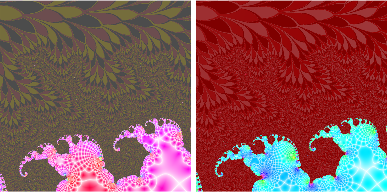
A different region
(The detailed code in this section is omitted in the post, but included in the attached notebook.)
Computing over a different region (-0.0452407411 + 0.9868162204352258 I + 2.7 10^-5 {-1 - I, 1 + I}) and fiddling with color palettes from ColorData["ThemeGradients"] gives us this wallpaper-like result (the ColorFunction used here is "M10DefaultDensityGradient").
Also the corresponding complex map plots:
References
 Attachments:


