A very neat idea, @Clayton, have not seen that yet around. Sooo it is that time of the year again when we get showered in code- and math- Xmas trees, awesome! I will post here a few the WL code for which I wrote the past. The first one comes from a very simple formula:
$$t * sin (t) ? Christmas Tree$$

It is a simple expanding 3D spiral and it is made with the following code:
PD = .5; s[t_, f_] := t^.6 - f;
 dt[cl_, ps_, sg_, hf_, dp_, f_] :=
    {PointSize[ps], Hue[cl, 1, .6 + sg .4 Sin[hf s[t, f]]],
     Point[{-sg s[t, f] Sin[s[t, f]], -sg s[t, f] Cos[s[t, f]], dp + s[t, f]}]};

 frames = ParallelTable[

    Graphics3D[Table[{dt[1, .01, -1, 1, 0, f], dt[.45, .01, 1, 1, 0, f],
                      dt[1, .005, -1, 4, .2, f], dt[.45, .005, 1, 4, .2, f]},
 {t, 0, 200, PD}],

     ViewPoint -> Left, BoxRatios -> {1, 1, 1.3}, ViewVertical -> {0, 0, -1},
    ViewCenter -> {{0.5, 0.5, 0.5}, {0.5, 0.55}}, Boxed -> False, Lighting -> "Neutral",
    PlotRange -> {{-20, 20}, {-20, 20}, {0, 20}}, Background -> Black],

   {f, 0, 1, .01}];

Export["tree.gif", frames]
Another one is made as ASCII art, which I really enjoy. Watch closely - the tree is also changing - snow sticks to branches then falls ;-)
To build it we start from simple observation that a bit of randomness builds a nice tree:
Column[Table[Row[RandomChoice[{"+", ".", "*", "~", "^", "o"}, k]], {k, 1, 35, 2}], Alignment -> Center]
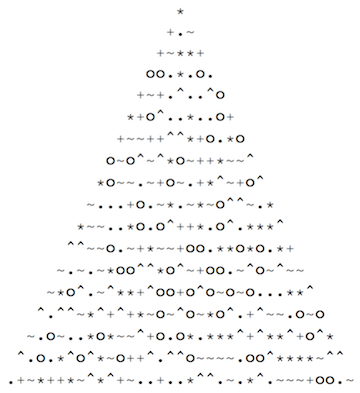
And now with a bit more sophistication a scalable dynamic ASCII tree:
DynamicModule[{atoms, tree, pos, snow, p = .8, sz = 15},

 atoms = {
   Style["+", White],
   Style["*", White],
   Style["o", White],
   Style[".", Green],
   Style["~", Green],
   Style["^", Green],
   Style["^", Green]
   };

 pos = Flatten[Table[{m, n}, {m, 18}, {n, 2 m - 1}], 1];

 tree = Table[RandomChoice[atoms, k], {k, 1, 35, 2}];

 snow = Table[
   RotateLeft[ArrayPad[{RandomChoice[atoms[[1 ;; 2]]]}, {0, sz}, " "],
     RandomInteger[sz]], {sz + 1}];

 Dynamic[Refresh[

   Overlay[{

     tree[[Sequence @@ RandomChoice[pos]]] = RandomChoice[atoms];
     Column[Row /@ tree, Alignment -> Center, Background -> Black],

     Grid[
      snow =
       RotateRight[
        RotateLeft[#,
           RandomChoice[{(1 - p)/2, p, (1 - p)/2} -> {-1, 0, 1}]] & /@
          snow
        , {1, 0}]]

     }, Alignment -> Center]

   , UpdateInterval -> 0, TrackedSymbols -> {}]
  ]
 ]
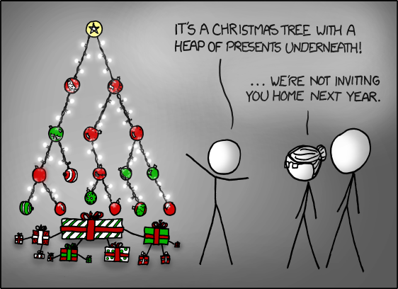
And the last one is not mine, but just to make you smile, from xkcd: