The ground state of a quantum mechanical problem can be found by minimizing the expectation value of the energy.
The first excited state can be found the same way, by making it orthogonal to the ground state, etc.
The following function takes three arguments, the potential energy function, the number of states to calculate and the spacing between the discretized values of x.
It returns a list of the energy of the states and a list of a list of the wavefunction values. It assumes [HBar]^2/(2m) = 1.
The second derivative in kinetic energy is approximated using a finite difference. The calculation is done between x = 0 and x = 1.
The optimization is performed using ParametricIPOPT, using a function defined in the attached notebook.
Only one random search (with random seed = 0)is needed for each energy level
cmpt[pefunc_, n_Integer, d_] :=
 Block[{i, vars, psi, vwb, ener, enres, varres, cons1, cons2, allcons,
    sln, wavefunctions},
  vars = Table[psi[x], {x, 0, 1, d}];
  vwb = {#, -5, 5} & /@ vars;
  ener = d Sum[-psi[x] ((psi[x + d] - 2*psi[x] + psi[x - d])/d^2) +
      psi[x] pefunc psi[x], {x, d, 1 - d, d}];
  enres = Table[0, n];
  varres = Table[0, n];
  wavefunctions = Table[0, n];
  cons1 = {psi[0] == 0, psi[1] == 0, vars.vars == d^-1};
  Do[cons2 = Table[vars.varres[[j]] == 0, {j, i - 1}];
   allcons = Join[cons1, cons2];
   sln = iMin[ener, allcons, vwb, 1, 0];
   enres[[i]] = sln[[1]];
   wavefunctions[[i]] = sln[[2]];
   varres[[i]] =  vars /. sln[[2]],
   {i, n}
   ]; {enres, wavefunctions}
  ]
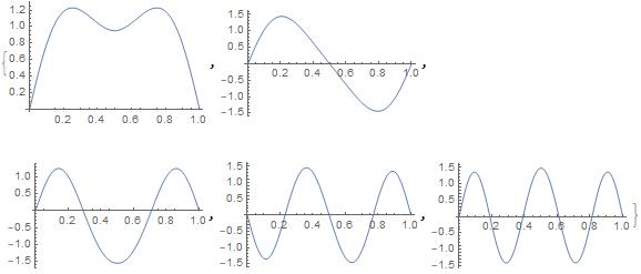
calculate energy levels and wavefunctions for first 5 states in an infinite square well potential with triangle potential inside.
In[6]:= tripot = cmpt[If[x < 1/2, 200*x, 200 (1 - x)], 5, 1/100];

During evaluation of In[6]:= {{Solve_Succeeded,1}}

During evaluation of In[6]:= {{Solve_Succeeded,1}}

During evaluation of In[6]:= {{Solve_Succeeded,1}}

During evaluation of In[6]:= {{Solve_Succeeded,1}}

During evaluation of In[6]:= {{Solve_Succeeded,1}}
energies
In[7]:= optenergies = tripot[[1]]

Out[7]= {73.9328, 86.7515, 144.504, 208.488, 297.988}
wavefunctions
In[8]:= Table[ListPlot[Table[{x, psi[x]}, {x, 0, 1, 1/100}] /. tripot[[2, n]],
  Joined -> True], {n, 5}]
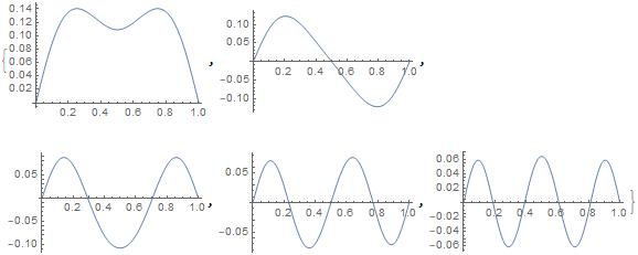
use energy levels found by optimization to solve Schrodinger's Equation, using ParametricNDSolve.
In[9]:= schrod = ParametricNDSolve[{-psi''[x] +
      If[x < 1/2, 200*x, 200 (1 - x)]*psi[x] == e psi[x], psi[0] == 0,
    psi'[0] == 1}, psi, {x, 0, 1}, {e}];
The energy levels from Schrodinger's Equation are close to those found using optimization.
In[10]:= schrodenergies = FindRoot[(psi[e][2] /. schrod) == 0, {e, #}] & /@ optenergies

Out[10]= {{e -> 73.9364}, {e -> 86.7689}, {e -> 144.564}, {e -> 208.699}, {e ->
   298.49}}
The wavefunctions found using Schrodinger's Equation are close to those found by optimization.
Note that these functions are not normalized, since the initial condition [Psi]'[0] == 1 was used.
Table[Plot[psi[e][x] /. schrod /. schrodenergies[[i]], {x, 0, 1}], {i,
   5}]
 Attachments:


