Introduction
This notebook / document provides ground data analysis used to make or confirm certain modeling conjectures and assumptions of a Pets Retail Dynamics Model (PRDM), [AA1]. Seattle pets licensing data is used, [SOD2].
We want to provide answers to the following questions.
Does the Pareto principle manifests for pets breeds?
Does the Pareto principle manifests for ZIP codes?
Is there an upward trend for becoming a pet owner?
All three questions have positive answers, assuming the retrieved data, [SOD2], is representative. See the last section for an additional discussion.
We also discuss pet adoption simulations that are done using Quantile Regression, [AA2, AAp1].
This notebook/document is part of the SystemsModeling at GitHub project "Pets retail dynamics", [AA1].
Data
The pet licensing data was taken from this page: Seattle Pet Licenses, https://data.seattle.gov/Community/Seattle-Pet-Licenses/jguv-t9rb/data.
The ZIP code coordinates data was taken from a GitHub repository,
"US Zip Codes from 2013 Government Data", https://gist.github.com/erichurst/7882666.
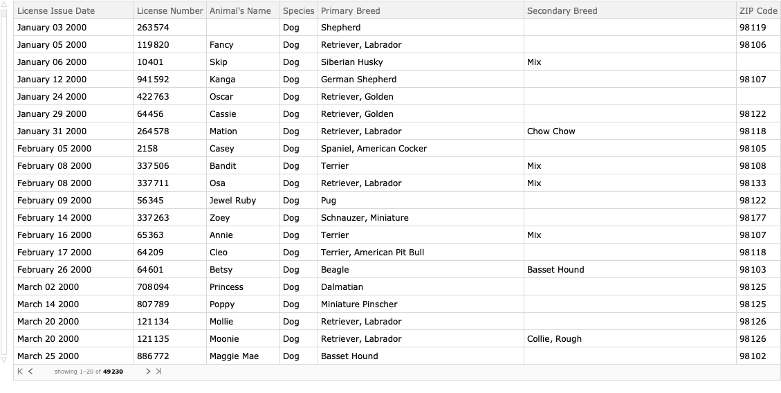
Animal licenses
dsPetLicenses=ResourceFunction["ImportCSVToDataset"]["~/Datasets/Seattle/Seattle_Pet_Licenses.csv"]
Convert Licence Issue Date values into DateObjects.
dsPetLicenses=dsPetLicenses[All,Prepend[#,"DateObject"->DateObject[{#[[1]],{"Month","Day","Year"}}]]&];
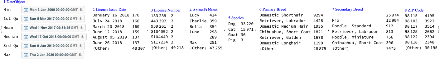
Summary
ResourceFunction["RecordsSummary"][dsPetLicenses]
Keep dogs and cats only
Since the number of animals that are not cats or dogs is very small we remove them from the data in order to produce more concise statistics.
dsPetLicenses=dsPetLicenses[Select[MemberQ[{"Cat","Dog"},#Species]&]];
    Dimensions[dsPetLicenses]

(*{49191,8}*)
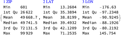
ZIP code geo-coordinates
dsZIPCodes=ImportCSVToDataset["~/Datasets/USAZipCodes/US-Zip-Codes-from-2013-Government-Data.csv"];
    Dimensions[dsZIPCodes]

(*{33144,3}*)
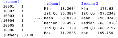
aZipLatLon=Association[Normal[Query[#ZIP->{#LAT,#LON}&]/@dsZIPCodes]];
    aZipLatLon=KeyMap[ToString,aZipLatLon];
    Length[aZipLatLon]

(*33144*)
Summary
ResourceFunction["RecordsSummary"][dsZIPCodes]
ResourceFunction["RecordsSummary"][aZipLatLon,Thread->True]
Pareto principle adherence
In this section we apply the Pareto principle statistic in order to see does the Pareto principle manifests over the different columns of the pet licensing data.
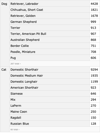
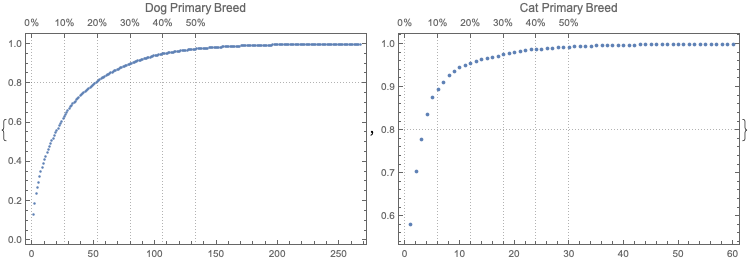
Breeds
We see a typical Pareto principle adherence for both dog breeds and cat breeds. For example, $20$% of the dog breeds correspond to $80$% of all registered dogs.
Note that the number of unique cat breeds is 4 times smaller than the number of unique dog breeds.
focusColumnName="Primary Breed";
dsQuery=Query[GroupBy[#Species&],GroupBy[#[focusColumnName]&],Length]@dsPetLicenses;
    dsQuery=Dataset[ReverseSort/@Normal[dsQuery]]
KeyValueMap[ResourceFunction["ParetoPrinciplePlot"][Values[#2],PlotLabel->Row[{#1,Spacer[3],focusColumnName}],ImageSize->Medium,opts]&,Normal[dsQuery]]
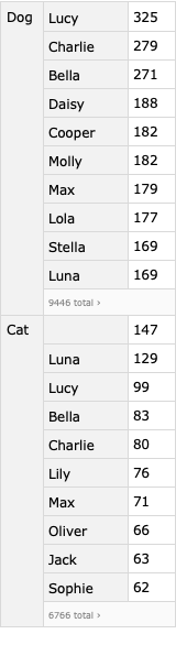
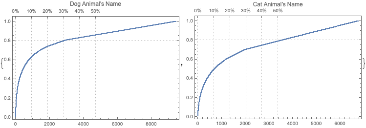
Animal names
We see a typical Pareto principle adherence for the frequencies of the pet names. For dogs, $10$% of the unique names correspond to ~ $65$% of the pets.
focusColumnName="Animal's Name";
dsQuery=Query[GroupBy[#Species&],GroupBy[#[focusColumnName]&],Length]@dsPetLicenses;
    dsQuery=Dataset[ReverseSort/@Normal[dsQuery]]
KeyValueMap[ResourceFunction["ParetoPrinciplePlot"][Values[#2],PlotLabel->Row[{#1,Spacer[3],focusColumnName}],ImageSize->Medium,opts]&,Normal[dsQuery]]
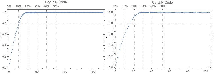
Zip codes
We see typical -- even exaggerated -- manifestation of the Pareto principle over ZIP codes of the registered pets.
focusColumnName="ZIP Code";
dsQuery=Query[GroupBy[#Species&],GroupBy[#[focusColumnName]&],Length]@dsPetLicenses;
    dsQuery=Dataset[ReverseSort/@Normal[dsQuery]];
KeyValueMap[ResourceFunction["ParetoPrinciplePlot"][Values[#2],PlotLabel->Row[{#1,Spacer[3],focusColumnName}],ImageSize->Medium,opts]&,Normal[dsQuery]]
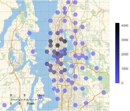
Geo-distribution
In this section we visualize the pets licensing geo-distribution with geo-histograms.
city=Entity["City",{"Seattle","Washington","UnitedStates"}];
    GeoPosition[city]

(*GeoPosition[{47.6205,-122.351}]*)
Both cats and dogs
lsCoords=Map[If[KeyExistsQ[aZipLatLon,#],aZipLatLon[#],Nothing]&,Select[ToString/@Normal[dsPetLicenses[All,"ZIP Code"]],StringQ[#]&&StringLength[#]>=5&]];
GeoHistogram[lsCoords,GeoCenter->city,GeoRange->Quantity[20,"Miles"],PlotLegends->Automatic,ColorFunction->(Hue[2/3,2/3,1-#]&),opts]
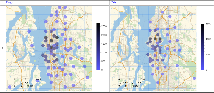
Dogs and cats separately
lsCoords=Map[If[KeyExistsQ[aZipLatLon,#],aZipLatLon[#],Nothing]&,Select[ToString/@Normal[dsPetLicenses[Select[#Species=="Dog"&],"ZIP Code"]],StringQ[#]&&StringLength[#]>=5&]];
    gr1=GeoHistogram[lsCoords,GeoCenter->city,GeoRange->Quantity[20,"Miles"],PlotLegends->Automatic,ColorFunction->(Hue[2/3,2/3,1-#]&),opts];
lsCoords=Map[If[KeyExistsQ[aZipLatLon,#],aZipLatLon[#],Nothing]&,Select[ToString/@Normal[dsPetLicenses[Select[#Species=="Cat"&],"ZIP Code"]],StringQ[#]&&StringLength[#]>=5&]];
    gr2=GeoHistogram[lsCoords,GeoCenter->city,GeoRange->Quantity[20,"Miles"],PlotLegends->Automatic,ColorFunction->(Hue[2/3,2/3,1-#]&),opts];
ResourceFunction["GridTableForm"][{gr1,gr2},TableHeadings->{"Dogs","Cats"},Background->White]
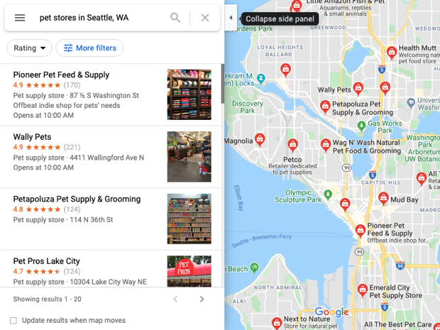
Pet stores
In this subsection we show the distribution of pet stores (in Seattle).
It is better instead of image retrieval to show corresponding geo-markers in the geo-histograms above. (This is not considered that important in the first version of this notebook/document.)
WebImage["https://www.google.com/maps/search/pet+stores+in+Seattle,+WA/@47.6326975,-122.4227211,12.05z"]
Time series
In this section we visualize the time series corresponding to the pet registrations.
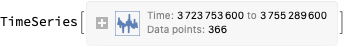
Time series objects
Here we make time series objects:
dsQuery=Query[GroupBy[#Species&],GroupBy[#DateObject&],Length]@dsPetLicenses;
    aTS=TimeSeries/@(List@@@Normal[#]&/@Normal[dsQuery])

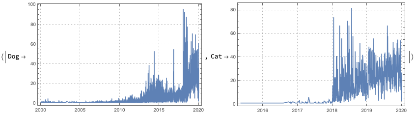
Time series plots of all registrations
Here are time series plots corresponding to all registrations:
DateListPlot[#,opts]&/@aTS
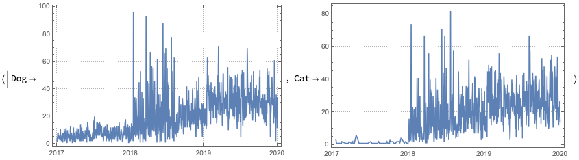
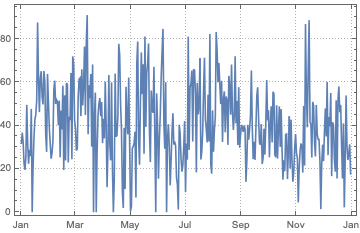
Time series plots of most recent registrations
It is an interesting question why the number of registrations is much higher in volume and frequency in the years 2018 and later.
DateListPlot[TimeSeriesWindow[#,{{2017,1,1},{2020,1,1}}],opts]&/@aTS
Upward trend
Here we apply both Linear Regression and Quantile Regression:
QRMonUnit[TimeSeriesWindow[#,{{2018,1,1},{2020,1,1}}]]?
    QRMonLeastSquaresFit[{1,x}]?
    QRMonQuantileRegressionFit[4,0.5]?
    QRMonDateListPlot[opts,"Echo"->False]?
    QRMonTakeValue&/@aTS
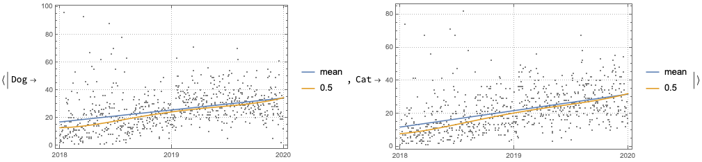
We can see that there is clear upward trend for both dogs and cats.
Quantile regression application
In this section we investigate the possibility to simulate the pet adoption rate. We plan to use simulations of the pet adoption rate in PRDM.
We do that using the software monad QRMon, [AAp1]. A list of steps follows.
Split the time series into windows corresponding to the years 2018 and 2019.
Find the difference between the two years.
Apply Quantile Regression to the difference using a reasonable grid of probabilities.
Simulate the difference.
Add the simulated difference to year 2019.
Simulation
In this sub-section we simulate the differences between the time series for 2018 and 2019, then we add the simulated difference to the time series of the year 2019.
ts1=TimeSeriesResample[TimeSeriesWindow[aTS[[1]],{{2018,1,1},{2019,1,1}}],"Day"];
    ts1["Path"][[All,2]];
ts2=TimeSeriesResample[TimeSeriesWindow[aTS[[1]],{{2019,1,1},{2020,1,1}}],"Day"];
    ts2["Path"][[All,2]];
ts3=TimeSeries[Transpose[{ts1["Path"][[All,1]],ts2["Path"][[All,2]]-ts1["Path"][[All,2]]}]]
qrObj=
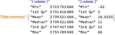
QRMonUnit[ts3]?
QRMonEchoDataSummary?
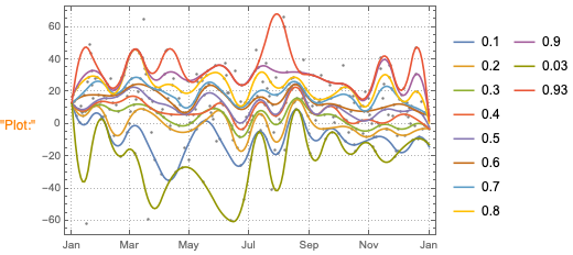
QRMonQuantileRegression[20,Join[Range[0.1,0.9,0.1],{0.03,0.93}],InterpolationOrder->2]?
QRMonDateListPlot[opts];
qrObj=
qrObj?
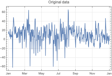
QRMonEchoFunctionContext[DateListPlot[#data,PlotLabel->"Original data",opts]&]?
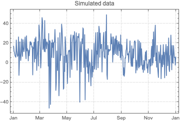
QRMonSimulate[ts2["Path"]//Length]?
QRMonEchoFunctionValue[DateListPlot[#,PlotLabel->"Simulated data",opts]&];
Take the simulated time series difference:
tsSimDiff=TimeSeries[qrObj?QRMonTakeValue];
Add the simulated time series difference to year 2019, clip the values less than zero, shift the result to 2020:
tsSim=MapThread[{#1[[1]],#1[[2]]+#2[[2]]}&,{ts2["Path"],tsSimDiff["Path"]}];
    tsSim[[All,2]]=Clip[tsSim[[All,2]],{0,Max[tsSim[[All,2]]]}];
    tsSim=TimeSeriesShift[TimeSeries[tsSim],Quantity[365,"Days"]];
    DateListPlot[tsSim,opts]
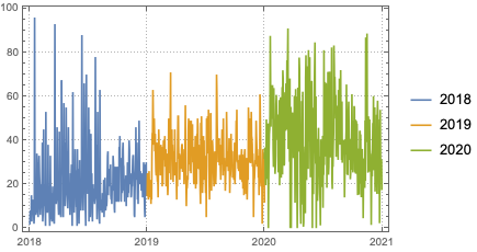
Plot all years together
DateListPlot[{ts1,ts2,tsSim},opts,PlotLegends->{2018,2019,2020}]
Discussion
This section has subsections that correspond to additional discussion questions. Not all questions are answered, the plan is to progressively answer the questions with the subsequent versions of the this notebook / document.
? Too few pets
The number of registered pets seems too few. Seattle is a large city with more than $600000$ citizens; approximately $50$% of the USA households have dogs; hence the registered pets are too few (~ $50000$).
? Why too few pets?
Seattle is a high tech city and its citizens are too busy to have pets?
Most people do not register their pets? (Very unlikely if they have used veterinary services.)
Incomplete data?
? Registration rates
Why the number of registrations is much higher in volume and frequency in the years 2018 and later?
? Adoption rates
Can we tell apart the adoption rates of pet-less people and people who already have pets?
Preliminary definitions
opts=Sequence@@{PlotRange->All,ImageSize->Medium,PlotTheme->"Detailed"};
Import["https://raw.githubusercontent.com/antononcube/MathematicaForPrediction/master/MonadicProgramming/MonadicQuantileRegression.m"]
References
[AA1] Anton Antonov, Pets retail dynamics project, (2020), SystemModeling at GitHub.
[AA2] Anton Antonov, A monad for Quantile Regression workflows, (2018), MathematicaForPrediction at WordPress.
[AAp1] Anton Antonov, Monadic Quantile Regression Mathematica package, (2018), MathematicaForPrediction at GitHub.
[SOD1] Seattle Open Data, Seattle Pet Licenses, https://data.seattle.gov/Community/Seattle-Pet-Licenses/jguv-t9rb/data .
 Attachments:


