Or you can actually fit a equation of a spiral to the given datapoints. To do so i converted the data points to polar coordinates (for which you need to define the center of the spiral).
I added three different spiral equations and some combination of those.
inp = N@adat;
(*center to first point*)
(*manually define center of spiral*)
first = {152, 172};(*mannulay defined center cooordinate*)
dat2 = # - first & /@ inp;
(*using first point as center*)
(*first=inp[[1]];
dat2=#-first&/@inp;
dat2=dat2[[2;;]];*)
(*convert to polar coordinates*)
rad = Norm /@ dat2;
ang = ArcTan @@@ dat2;
(*unwrap the angles - order is important*)
angs = ang +
Prepend[-2 Pi (Accumulate[Floor[Abs[Differences[ang]]/(1.5 Pi)]]),
0];
(*make all angles positve*)
angs = angs - Floor[Min[angs], 2 Pi];
ListLinePlot[{angs, ang}, PlotLegends -> {"unwrapped", "wrapped"}]
(*define fit data*)
fdat = SortBy[Transpose[{angs, rad}], First];
(*define models*)
model1 = a Exp[Cot[b] \[Phi]];(*logarithmic spiral*)
model2 = a + b \[Phi]; (*archimedean spiral*)
model3 = a + b/\[Phi]; (*eqation in notebook*)
(*combination of the different models*)
modelf1 = a1 Exp[Cot[b1] \[Phi]] + a2 + b2 \[Phi];
modelf2 = a1 Exp[Cot[b1] \[Phi]] + a2 + b2 /\[Phi];
modelf3 = a1 Exp[Cot[b1] \[Phi]] + a2 + b2 \[Phi] + b3 /\[Phi];
(*find the fit for each model*)
sol1 = FindFit[fdat, model1, {a, b}, \[Phi]];
sol2 = FindFit[fdat, model2, {a, b}, \[Phi]];
sol3 = FindFit[fdat, model3, {a, b}, \[Phi]];
solf1 = FindFit[fdat, modelf1, {a1, b1, a2, b2}, \[Phi]];
solf2 = FindFit[fdat, modelf2, {a1, b1, a2, b2}, \[Phi]];
solf3 = FindFit[fdat, modelf3, {a1, b1, a2, b2, b3}, \[Phi]];
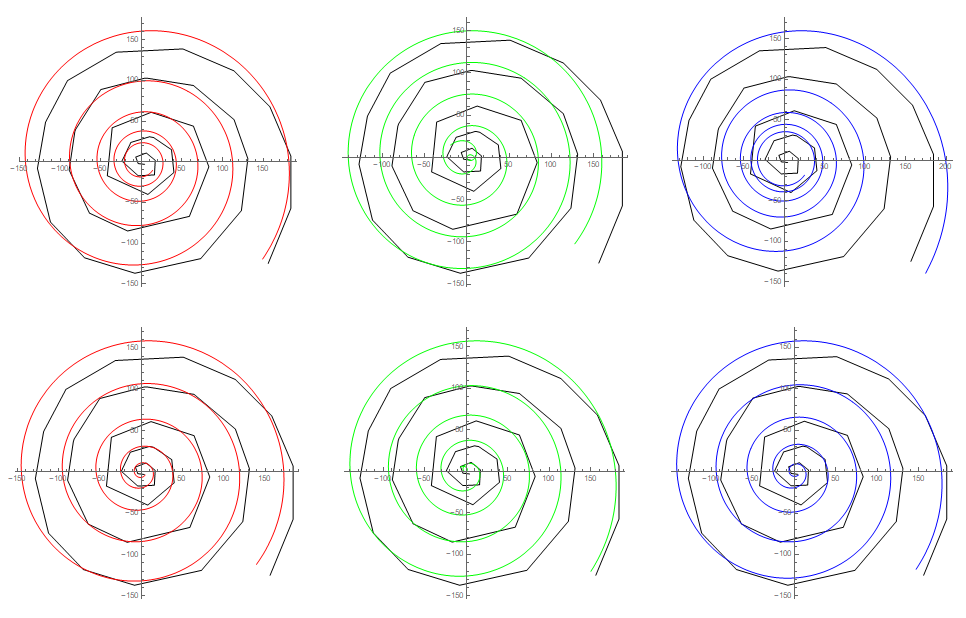
(*make plots*)
p0 = ListPolarPlot[fdat, Joined -> True, PlotStyle -> Black];
p1 = PolarPlot[(model1 /. sol1), {\[Phi], Min[angs], Max[angs]},
PlotStyle -> Red];
p2 = PolarPlot[(model2 /. sol2), {\[Phi], Min[angs], Max[angs]},
PlotStyle -> Green];
p3 = PolarPlot[(model3 /. sol3), {\[Phi], Min[angs], Max[angs]},
PlotStyle -> Blue];
GraphicsRow[Show[p0, #, PlotRange -> Full] & /@ {p1, p2, p3},
ImageSize -> 1200]
(*make plots combined models*)
p0 = ListPolarPlot[fdat, Joined -> True, PlotStyle -> Black];
p1 = PolarPlot[(modelf1 /. solf1), {\[Phi], Min[angs], Max[angs]},
PlotStyle -> Red];
p2 = PolarPlot[(modelf2 /. solf2), {\[Phi], Min[angs], Max[angs]},
PlotStyle -> Green];
p3 = PolarPlot[(modelf3 /. solf3), {\[Phi], Min[angs], Max[angs]},
PlotStyle -> Blue];
GraphicsRow[Show[p0, #, PlotRange -> Full] & /@ {p1, p2, p3},
ImageSize -> 1200]
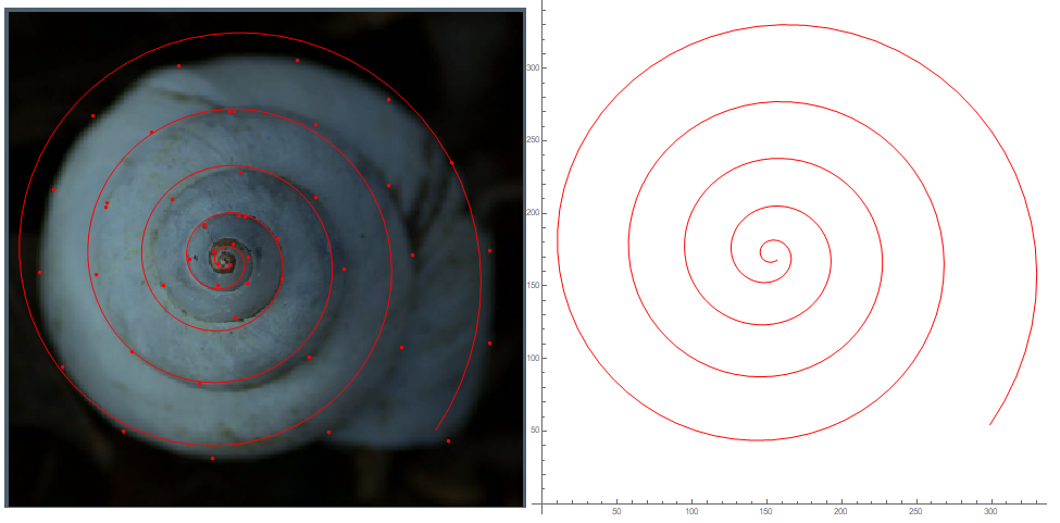
(*show "best model"*)
{modelBest, solBest} = {modelf3, solf3};
FullSimplify[modelBest /. solBest]
pBest = ListLinePlot[
Transpose[({Cos[\[Phi]] modelBest, Sin[\[Phi]] modelBest} +
first /. solBest) /. \[Phi] ->
Range[Min[angs], Max[angs], .1]], PlotStyle -> Red,
ImageSize -> 600, AspectRatio -> 1];
Row[{Show[img, ListPlot[inp, PlotStyle -> {PointSize[Medium], Red}],
pBest, ImageSize -> 600], pBest}]