Message Boards Message Boards

[GIF] Nines (Minimum-stick 9-crossing knots)

Minimum-stick 9-crossing knots

Nines

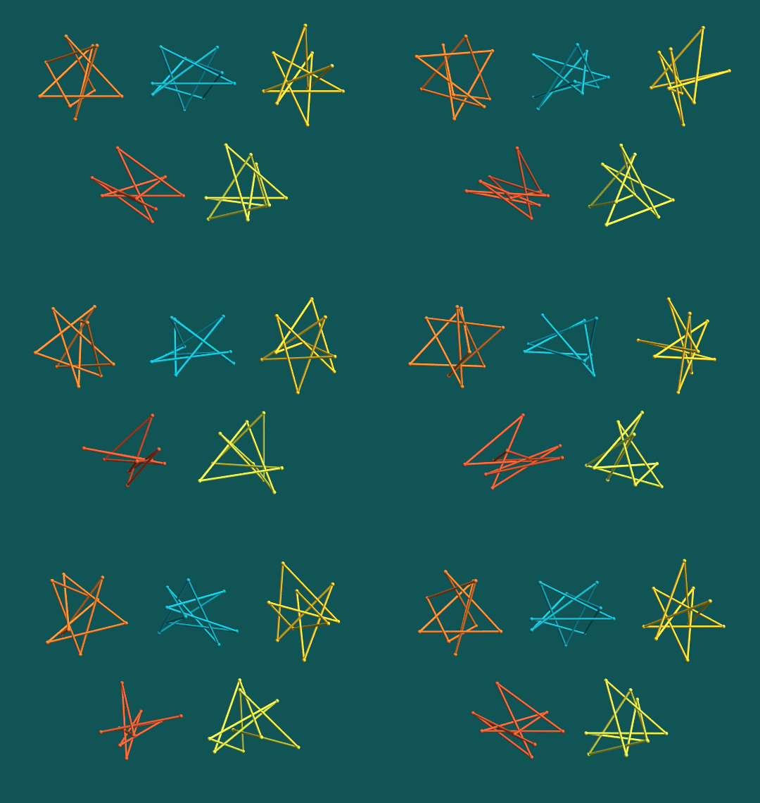
In our paper "New stick number bounds from random sampling of confined polygons", my graduate student Thomas D. Eddy and I found many examples of polygonal knots made with fewer edges than previously observed. Among these, we found 9-edge examples of the knots $9_{35}$, $9_{39}$, $9_{43}$, $9_{45}$, and $9_{48}$. Since these knots were already previously known to require at least 9 edges, this proved that the stick number (minimum number of edges needed) for these knots is exactly 9.

In addition to the results in the paper, we provide both source code and data on Github; among the data are the current best bounds on stick number for all knots up to 10 crossings and coordinates of vertices achieving these bounds.

The animation shows each of the five knots $9_{35}$, $9_{39}$, $9_{43}$, $9_{45}$, and $9_{48}$ in the minimal configuration we discovered.

To make the animation, first extract coordinates from Github:

knotcoords = 
  Import["https://raw.githubusercontent.com/thomaseddy/stick-knot-gen/\
master/data/mseq_knots/" <> # <> ".txt", "Data"] & /@
   {"9_35", "9_39", "9_43", "9_45", "9_48"};

Next, some functions for mean-centering and offsetting a collection of points:

MeanCenter[p_] := Table[p[[i]] - Mean[p], {i, 1, Length[p]}];
HorizontalOffset[p_, v_] := Table[p[[i]] + v, {i, 1, Length[p]}];

And some specific offsets for making this particular animation, found mostly by trial and error:

offsets = 1.4 {{-1, 1/2, 0}, {0, 1/2, 0}, {1, 1/2, 0}, {-1/2, -1/2, 0}, {1/2, -1/2, 0}};

And then here's a Manipulate for the animation (see this comment for the process of exporting to GIF):

DynamicModule[{p, 
  cols = RGBColor /@ {"#D9782D", "#12A4B6", "#ECC530", "#CC5430", 
     "#C9D845", "#105456"}},
 Manipulate[
  Show[
   Table[
    p = HorizontalOffset[
      MeanCenter[
       knotcoords[[i]].RotationMatrix[-θ, {0, 1, 0}]], offsets[[i]]];
    Graphics3D[{cols[[i]], Tube[Append[#, #[[1]]], .015] &[p], 
      Sphere[#, .025] & /@ p},
     Boxed -> False, SphericalRegion -> True, PlotRange -> 2, 
     ViewAngle -> π/8, ViewPoint -> Top],
    {i, 1, 5}],
   ImageSize -> {540, 400}, Background -> cols[[-1]], Lighting -> "Neutral"],
  {θ, 0, 2 π}]
 ]

If you want to know more, but don't want to read our whole paper, check out these slides for a talk that was cancelled due to COVID–19 concerns after I had already written the slides.

2 Replies

enter image description here -- you have earned Featured Contributor Badge enter image description here

Your exceptional post has been selected for our editorial column Staff Picks http://wolfr.am/StaffPicks and Your Profile is now distinguished by a Featured Contributor Badge and is displayed on the Featured Contributor Board. Thank you, keep it coming, and consider contributing to the The Notebook Archive!

POSTED BY: Moderation Team
Posted 4 years ago

Here's a slightly simplified version of Clayton's original implementation:

knotcoords = Table[Import["https://raw.githubusercontent.com/thomaseddy/stick-knot-gen/master/data/mseq_knots/9_"
                          <> IntegerString[k] <> ".txt", "Data"],
                   {k, {35, 39, 43, 45, 48}}];

offsets = 1.4 {{-1, 1/2, 0}, {0, 1/2, 0}, {1, 1/2, 0}, {-1/2, -1/2, 0}, {1/2, -1/2, 0}};

DynamicModule[{p, cols = RGBColor /@ {"#D9782D", "#12A4B6", "#ECC530",
                                      "#CC5430", "#C9D845", "#105456"}}, 
              Manipulate[Graphics3D[MapThread[
                         Function[{cl, kn, of}, GraphicsComplex[
                         TranslationTransform[of][Standardize[kn .
                                                  RotationMatrix[-θ, {0, 1, 0}],
                                                  Mean, 1 &]],
                         {cl, Tube[Append[Range[Length[kn]], 1], 0.015], 
                          Sphere[Range[Length[kn]], .025]}]],
                         {Most[cols], knotcoords, offsets}],
                         Boxed -> False, SphericalRegion -> True, PlotRange -> 2,
                         ViewAngle -> π/8, ViewPoint -> Top, ImageSize -> {540, 400},
                         Background -> cols[[-1]], Lighting -> "Neutral"],
                         {θ, 0, 2 π}, SaveDefinitions -> True]]

Some notes:

  • MeanCenter[] and HorizontalOffset[] were replaced with the built-ins Standardize[] and TranslationTransform[].

  • GraphicsComplex[] is useful for sharing points between the Sphere[] and Tube[] objects. Sphere[]'s first argument can be a list of centers, such that all those spheres have a fixed radius.

  • Instead of using Table[] and looping over different lists of the same length, it can be more convenient to use MapThread[].

POSTED BY: J. M.
Reply to this discussion
Community posts can be styled and formatted using the Markdown syntax.
Reply Preview
Attachments
Remove
or Discard

Group Abstract Group Abstract