Hello,
I like these elegant BarChart solutions. I’m a beginner and took a more “direct” approach. But then I thought how to bring some uniqueness to the solution. I thought it would be cool to use a speech synthesizer that verbalizes the height of the histogram bars. I found a speech synthesizer but the problem I face is how to take the adjustable bar height numerical value; convert it to text; and have the text inserted into the speech synthesizer. Any suggestions would be very helpful . I've attached my bar-chart program. Thank you very much,
Andrew Skipor
Daily Challenge (Day 12): Share with us an interesting piece of data visualization from your work/study/reasearch.
|
|
Here's mine:
Manipulate[
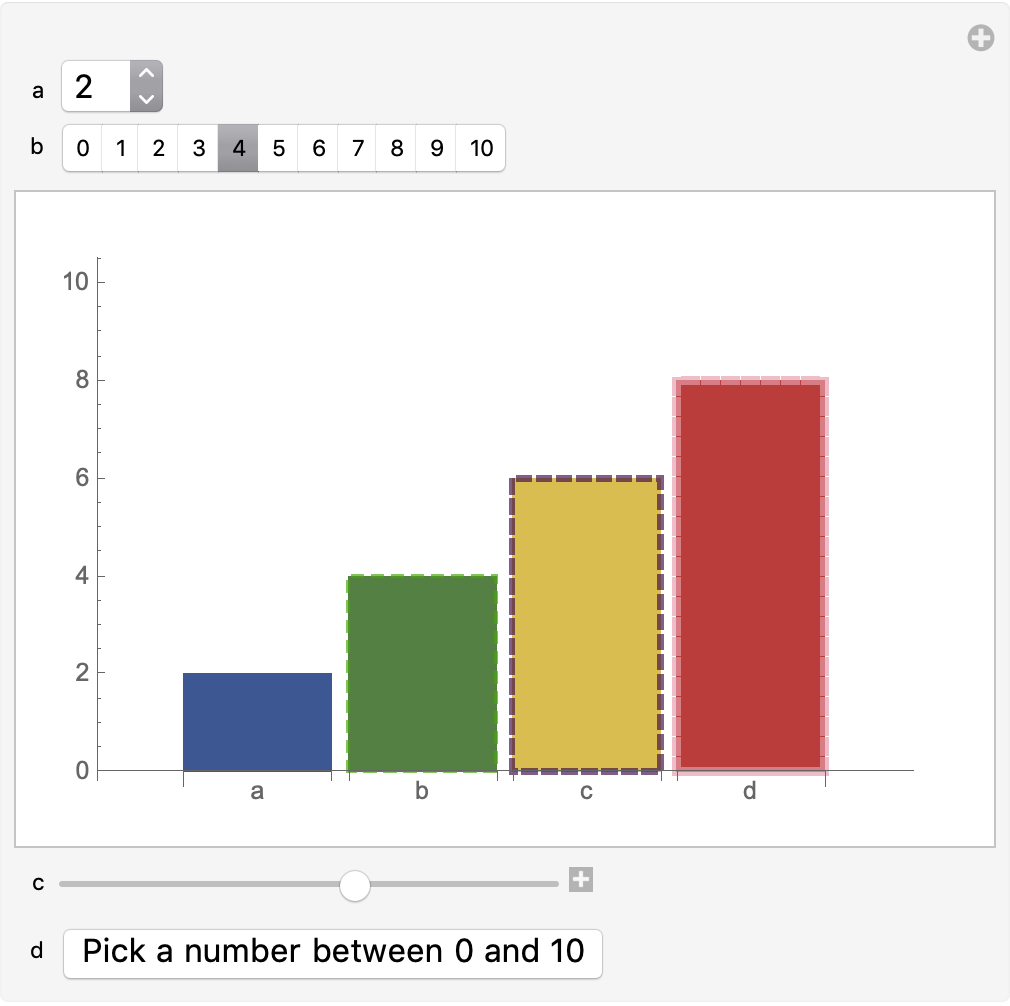
BarChart[{a, b, c, d}, ChartStyle -> "DarkRainbow",
ColorFunction ->
Function[{x},
Directive[ ColorData["DarkRainbow"][x],
EdgeForm[{Thickness[x/100], Dashed, RandomColor[]}]]],
ChartLabels -> {"a", "b", "c", "d"}, PlotRange -> {0, 10},
ImagePadding -> 10], {{a, 2}, Range[0, 10]}, {{b, 4}, Range[0, 10],
ControlType -> SetterBar}, {{c, 6}, 0, 10, 1}, {{d, 8},
Button["Pick a number between 0 and 10",
d = RandomInteger[{0, 10}]] &},
ControlPlacement -> {Top, Top, Bottom, Bottom}]

|
|
Manipulate[
BarChart[{a[[1]], a[[2]], b[[1]], b[[2]]},
ChartLabels -> {"\!\(\*SubscriptBox[\(a\), \(1\)]\)",
"\!\(\*SubscriptBox[\(a\), \(2\)]\)",
"\!\(\*SubscriptBox[\(b\), \(1\)]\)",
"\!\(\*SubscriptBox[\(b\), \(2\)]\)"}, LabelingFunction -> Above,
PlotRange -> {-0.5, 10.2}, ChartElementFunction -> "GlassRectangle",
ChartStyle -> "Pastel", PlotTheme -> "Business"],
Row[{Control[{{a, {3, 1}}, {0, 0}, {10, 10},
Appearance -> "Labeled"}],
Control[{{b, {7, 10}}, {0, 0}, {10, 10},
Appearance -> "Labeled"}]}]]

|
|
Manipulate[
BarChart[{a, b, c, d},
PlotRange -> {0, 10},
LabelingFunction -> Top,
ChartLabels -> Placed[{"a", "b", "c", "d"}, Above],
ColorFunction -> "Rainbow"],
{a, 0, 10}, {b, 0, 10}, {c, 0, 10}, {d, 0, 10}]

|
|
Manipulate[
BarChart[{b1, b2, b3, b4}, LabelingFunction -> Center,
PlotRange -> {All, {0, 10}}],
Row[{
Control[{{b1, 0, "b1"}, 0, 10, 1, Appearance -> "Labeled"}],
Control[{{b2, 0, "b2"}, 0, 10, 1, Appearance -> "Labeled"}],
Control[{{b3, 0, "b3"}, 0, 10, 1, Appearance -> "Labeled"}],
Control[{{b4, 0, "b4"}, 0, 10, 1, Appearance -> "Labeled"}]
}],
ControlPlacement -> Right, ControlType -> VerticalSlider
]

|
|
Daily Challenge (Day 12): This one is again from EIWL (Chapter 9). Make a Manipulate to show a bar chart with 4 bars, each with a height that can be between 0 and 10
|
|
Thanks for the amazing contour plots!!!
Remember no study group today but please feel free to check out the second session of our "New in Wolfram Language 12.1" webinar series at
|
|
(*A little bit memory intensive but nice*)
threeLavaredoPeaks =
GeoElevationData[Entity["Mountain", "TreCimeDiLavaredo"],
GeoRange -> Quantity[5, "Kilometers"],
GeoProjection -> Automatic, GeoZoomLevel -> 12] // Reverse;
(*Plots. Mouse over contour line will show tooltip with height value*)
GraphicsRow[{
GeoContourPlot[
Reverse@GeoElevationData[
GeoBoundingBox[
GeoDisk[Entity["Mountain", "TreCimeDiLavaredo"],
Quantity[5, "Kilometers"]]], Automatic, "GeoPosition",
GeoZoomLevel -> 12], GeoBackground -> "Satellite",
ContourStyle -> White, ImageSize -> 450],
ListContourPlot[threeLavaredoPeaks, ColorFunction -> "DarkTerrain",
ContourLabels -> Automatic, ImageSize -> 600],
ReliefPlot[threeLavaredoPeaks, ColorFunction -> "DarkTerrain",
ImageSize -> 550]
}, Spacings -> {10, 0}, ImageSize -> 1000]

(*3D plot*)
ListPlot3D[threeLavaredoPeaks, Mesh -> None,
ColorFunction -> "DarkTerrain", ImageSize -> 900]

|
|
elevations =
GeoElevationData[
GeoBoundingBox@
GeoDisk[Entity["Mountain", "Moldoveanu"],
Quantity[5, "Kilometers"]], Automatic, "GeoPosition",
GeoZoomLevel -> 10];
GeoContourPlot[elevations, GeoBackground -> "ReliefMap",
ContourShading -> True, ColorFunction -> Hue,
PlotLegends -> Automatic]

|
|
nearestMountain = GeoNearest["Mountain", Here] // First;
elevationData =
GeoElevationData[nearestMountain,
GeoRange -> Quantity[5, "Kilometers"],
UnitSystem -> "Metric"];
ListContourPlot[Reverse@elevationData, ColorFunction -> "LightTerrain"]

Turns out that the mountain nearest me has higher elevations within 5 km than the mountain itself.
|
|
Daily challenge (Day 11): Create a contour plot of a 5 km radius around the nearest mountain peak to wherever you are situated.
|
|
Graphics[{Table[{Opacity[0.2], RandomColor[],
EdgeForm[
Directive[Opacity[.3], Dashed,
Thickness[RandomReal[{0.05, 0.1}]], RandomColor[]]],
Disk[RandomReal[10, 2], RandomReal[{.5, 1.}]]}, {200}]}]

|
|
Hi, Abrita, I have modified a little your code:
Graphics[Table[{RGBColor[i^2/100, j^2/100, 1 - (i^2 + j^2)/200],
EdgeForm[
Directive[Opacity[.977], Dashed,
Thickness[RandomReal[{0.05, 0.1}]], Opacity[.87],
Hue[(i^2 + j^2)/200]]], Disk[{i, j}, RandomReal[{.5, 1.}]]}, {i,
10}, {j, 10}]]
to obtain the following result: 
|
|
A simple modification of an example from the EIWL:
Style[Circle[{#, 0}, #], Hue[0.01 #^2]] & /@ Range[0, 10, .01] // Graphics

or
Style[Circle[{0.1 Cos@#, 0.9 Sin@#}, #], Hue[0.0091 #^2]] & /@
Range[0, 11.5, .01] // Graphics

|
|
Stephen Wolfram is a colorful character.
sw = Entity["PopularCurve", "StephenWolframCurve"]["Graphics"];
SeedRandom[314];
sw /. RGBColor[___] :> RandomColor[] /. AbsoluteThickness[1] -> AbsoluteThickness[2] /.
Axes -> False

|
|
Hello,
These are representations of a scaling of the solar system over a GAA pitch and the scaling of some incidents of the timeline of the Universe over a GAA pitch that I made for a quarantine quiz with friends over the weekend. GAA is the governing organisation covering some Irish sports. Hurling and Gaelic Football are played on these style pitches. Whenever we get back to training and playing matches now, hopefully I will also be revising my appreciation for these scales of our existence. I'll add more elements in future but that should be quite straightforward now hopefully. Donnacha
|
|
Reply to this discussion
in reply to
|