Intending a differential equation model of COVID-19 to estimate the termination states of disasters. In the other reports, Gompertz curve model was introduced however only the case of Japan, could not match any model to the trend in Japan. Recently, Japan national institute confirmed that Japan had infected serially by two major viruses. Following the information, it was found that the case of Japan can be illustrated with the conjunction of two Gompertz curves. Basics of the idea and deployments is illustrated in a slide file in Japanese.

Principal is straightforward one. First step is to divide the death number trend into the first and second part. Applying Gompertz equation to the first trend and obtain a curve F, then subtract F from the raw trend to obtain second infection trend. Applying Gompertz equation to the second trend which is free from the first infection effect, and obtain a curve L. A curve F+L is the intended answer.

1) obtain trend of Japan

    country = "Japan";
    urlCovid19 = "https://pomber.github.io/covid19/timeseries.json"; data \
    = Map[Association, Association[Import[urlCovid19]][country], {1}];
    ddata = {DateObject[#["date"]], #["deaths"]} & /@ data;
    firstday = ddata[[1, 1]];
    Last[ddata]

2) get data for the estimation

    i3 = Map[{QuantityMagnitude[#[[1]] - firstday], #[[2]]} &, ddata];
    i4 = Map[First, Gather[i3, #1[[2]] == #2[[2]] &]];
    ListPlot[i4]

3) get first part, where dividing report day is 70

    i5 = Select[i4, #[[1]] <= 70 &];

4) set initial guess for the first part

    start = 40;
    model0 = n b^Exp[-c ( t - start)];
    initialguess = {n -> 500, c -> 0.02, b -> 0.01};
    Show[
     Plot[model0 /. initialguess, {t, 0, 1000}, 
      PlotRange -> {{0, 150}, {0, 200}}],
     ListPlot[i5]
     ]

5) estimate a Gompertz curve fitted

    ans = FindFit[i5, model0, initialguess /. Rule -> List, t, 
      MaxIterations -> 200]

6) obtain second part subtracted the effect of first part

    pdays = First[Transpose[i4]];
    death = Last[Transpose[i4]];
    ListPlot[diff = 
      Transpose@{pdays, death - (model0 /. ans /. t -> pdays)}]

7) set initial guess of subtracted second part

    start = 80;
    model1 = n b^Exp[-c ( t - start)];
    initialguess = {n -> 500, c -> 0.1, b -> 0.01};
    Show[
     Plot[model1 /. initialguess, {t, 0, 1000}, 
      PlotRange -> {{0, 150}, {0, 800}}],
     ListPlot[diff]
     ]

8) get Gompertz curve fitted

    ans3 = FindFit[diff, model1, initialguess /. Rule -> List, t, 
      MaxIterations -> 400]

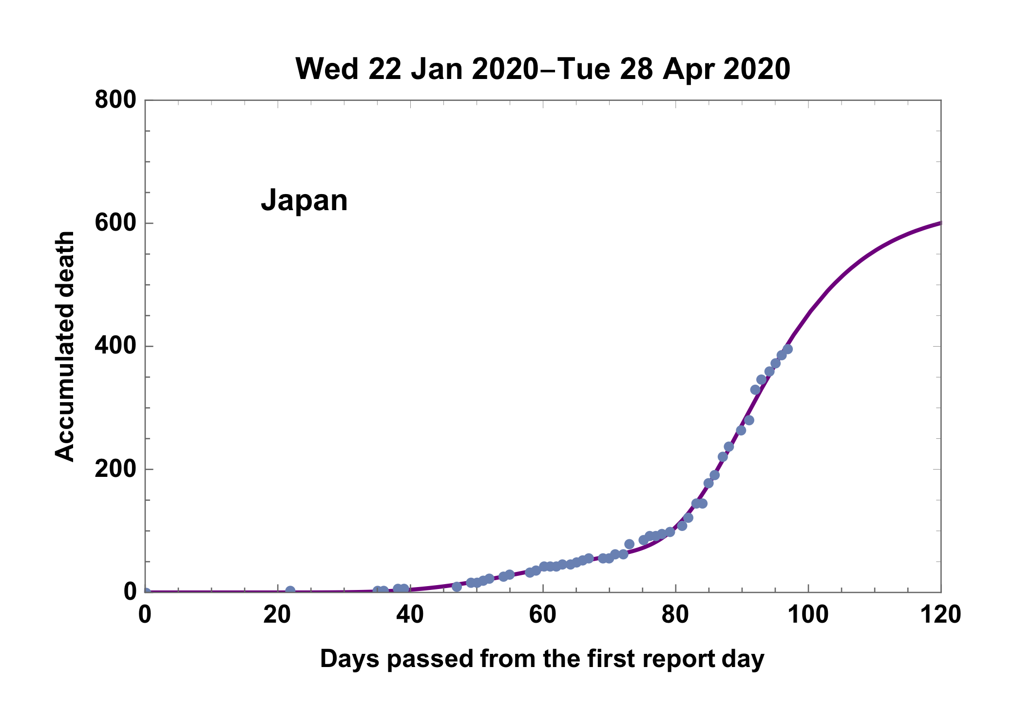
9) Finally obtained curve and reported death number of Japan

    fdate = First[ddata][[1]];
    ldate = Last[ddata][[1]];
    upto = 120;

    Show[
     Plot[(model0 /. ans) + (model1 /. ans3), {t, 0, upto}, 
      PlotRange -> {{0, upto}, {0, 800}}, PlotStyle -> {Purple}],
     ListPlot[i4, 
      PlotLegends -> Placed[Text[Style[country, Bold]], {0.2, 0.8}]],
     PlotRange -> {{0, upto}, {0, 800}},

     ImageMargins -> 20,
     Frame -> True,
     PlotLabel -> DateString[fdate] <> "-" <> DateString[ldate],
     FrameLabel -> {"Days passed from the first report day", 
       "Accumulated death"}, LabelStyle -> {Black}]