Attainment:
Mathematica has been a great source of inspiration and creativity for me. After two weeks of examination rounds by an extremely demanding and specialized team from the OEIS (The-Online Encyclopedia of Integer Sequences), my new sequences were finally approved and I managed to publish two more sequences. Many thanks to everyone involved and special thanks to Wolfram.
In this work, I analyze, with Wolfram Language, the two sequences, exposing their properties, characteristics, interesting facts and discuss the behaviors and their differences.
OEIS sequence descriptions:
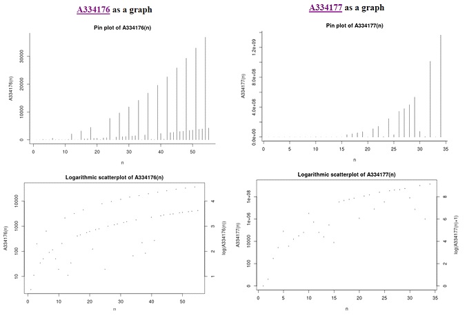
- A334176-OEIS: “Squarefree part of numerator of the squared area of the Heronian triangle with sequential odd sides whose shortest leg is 2 n+1.” – May 01, 2020. Autor: Claudio Lobo Chaib Filho (Mathematica, April 17, 2020). Colaboration: Michel Marcus (PARI code, April 18 2020) e Bernard Schott (formula using “core (squarefree)” sequence (A007913), April 18 2020).
Description: These are the values within the irreducible square roots, which are part of the area resulting from Heronian triangles, which have all sides being sequential odd integers (starting with the second odd number, since the triangle {1,3,5} has no real area). The triangles follow this sequence of sides: {2 n+1, 2n+3, 2n+5} and their area is represented by {(r/s) sqrt(t)}, where r, s, t are integers and a(n) is the number t.
Example: a(1) = 3 because the first possible Heronian triangle with its sequential odd integer sides is the triangle {3,5,7} and its respective area is {15 sqrt(3)/4}. a(2) = 11 since the second possible triangle is {5,7,9} which has area {21 sqrt(11)/4}. And so on.
- A334177-OEIS: “Squarefree part of numerator of the squared area of the Heronian triangle with sequential prime sides whose shortest leg is prime(n).” – May 01, 2020. Autor: Claudio Lobo Chaib Filho (Mathematica, April 17, 2020). Colaboration: Michel Marcus (PARI code, April 18 2020).
Description: These are the values within the irreducible square roots, which are part of the area resulting from Heronian triangles, which have all sides being sequential prime numbers. The triangles follow this sequence of sides: {prime(n), prime(n+1), prime(n+2)} and their area is represented by {(r/s) sqrt(t)}, where r, s, t are integers and a(n) is the number t.
Example: a(1) = 0, since the triangle {2,3,5} has area 0. a(2) = 3, because the first possible Heronian triangle with sequential prime sides and positive area is the triangle {3,5,7} and its respective area is {15 sqrt(3)/4}. a(3) = 299 since the second possible triangle is {5,7,11} which has area {3 sqrt(299)/4}. And so on.
For those who are not familiar with OEIS, on its page, we can hear the sound that a specific sequence produces. Run the code below and access the links to hear the sound of the A334176 and A334177:
HTTPRequest["https://oeis.org/play?seq=A334176"]
HTTPRequest["https://oeis.org/play?seq=A334177"]
Sequence Exploration:
- Personal analysis of the sequences:
These are the codes using Mathematica to produce these sequences, I call A334176: “aodd”, and I call A334177: “aprime”:
(* A334176-OEIS *)
aodd[n_] :=
 Module[{y, z},
  z = Area@SSSTriangle[2*n + 1, 2*n + 3,
     2*n + 5]; ({z} /.
      Coefficient[{z} /. Sqrt[_] -> y, y][[1]] -> 1)[[1]]^2]

(* A334177-OEIS *)
aprime[n_] :=
 Module[{y, z},
  If[n == 1, 0,
   z = Area@
     SSSTriangle[Prime[n], Prime[n + 1],
      Prime[n + 2]]; ({z} /.
       Coefficient[{z} /. Sqrt[_] -> y, y][[1]] -> 1)[[1]]^2]]
The first terms:
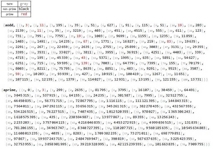
As seen above, the two sequences have only odd terms. "aodd" has a certain frequency for prime results, (in 100000 terms, 143 are prime), while "aprime" does not have any prime term in 100000 terms, with the exception of the 2nd term (number 3).
Creating a sample for analysis:
{odd0, odd, prime0, prime} = {Table[aodd[i], {i, 1, 100}],
   Table[aodd[i], {i, 1, 2000}], Table[aprime[i], {i, 1, 100}],
   Table[aprime[i], {i, 1, 2000}]};
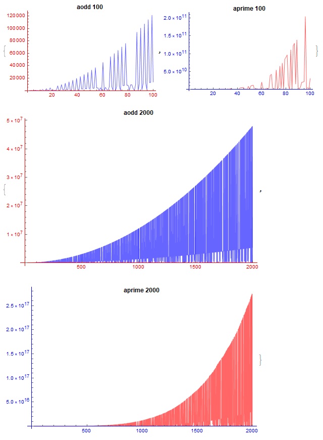
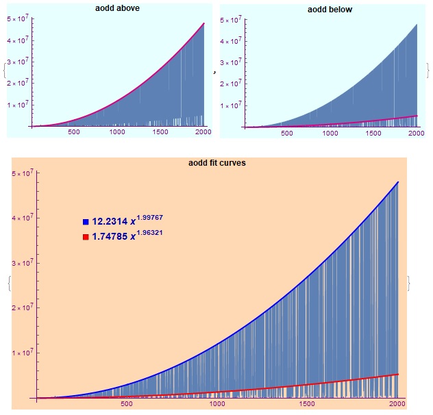
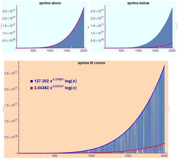
The first 100 terms and the first 2000 terms are presented below. Note that their behavior, despite being similar in some aspects, has different models: “aodd” is governed by a {a x^b} model and “aprime” is governed by a {a x^b log(x)} model.
Another striking feature that can be distinguished, especially for many terms exposed, is that there are two visible separations, one at the top of the graph and one at near the bottom of the graph.
afunct[type_] :=
 Module[{a, b, c},
  c = {"odd0", "prime0", "odd", "prime"}; {a, b} = {Blue, Red};
  ListLinePlot[ToExpression[type], PlotRange -> All,
   PlotStyle ->
    Directive[type /. AssociationThread[c -> {a, b, a, b}],
     Opacity[0.6]],
   AxesStyle -> type /. AssociationThread[c -> {b, a, b, a}],
   ImageSize -> type /. {"odd0" | "prime0" -> 300,
     "odd" | "prime" -> 500},
   PlotLabel ->
    Style[type /.
      AssociationThread[
       c -> {"aodd 100", "aprime 100", "aodd 2000", "aprime 2000"}],
     Black, Bold]]]
{afunct["odd0"], afunct["prime0"]}
{afunct["odd"], afunct["prime"]}
Fitting:
To analyze the behavior of the sequences, I created models that fit these separations (in many of the analysis here, I disregarded the initial 0 for “aprime”):
afit[type_, h_ : 1] :=
 Module[{aa, c1, o, data, m1, f1, mf1, r1, r2, r3, r4, r5, f2, mf2,
   g}, Clear[a, b, x]; aa = ToExpression[type];
  c1 = Map[Max[#] &, Partition[aa, 20]];
  o = {{a, b}, WorkingPrecision -> 50, MaxIterations -> 1000};
  data = Thread[{Table[
      Position[aa, c1[[j]]][[1, 1]], {j, 1, Length@c1}], c1}];
  m1 = type /. {"odd" -> (a *x^b), "prime" -> (a*x^b*Log[x])};
  f1 = FindFit[data, m1, o[[1]], x, o[[2]], o[[3]]];
  mf1 = Function[{x}, Evaluate[m1 /. f1]];
  r1 = Table[
    If[aa[[k]] < (0.15*(mf1[[2]] /. {x -> k})),
     Thread[{Position[aa, aa[[k]]][[1, 1]], aa[[k]]}], Nothing], {k,
     1, Length@aa}]; r2 = Table[r1[[v, 2]], {v, 1, Length@r1}];
  r3 = Select[
    Normal[Counts@Join[r2, Map[Min[#] &, Partition[r2, 2]]]],
    Last@# <= 1 &];
  r4 = Table[
    If[(Keys@r3)[[k]] >
      ToExpression[type /. {"odd" -> 1, "prime" -> h}]*
       Mean@Keys@r3, (Keys@r3)[[k]], Nothing], {k, 1, Length@r3}];
  r5 = Table[{Position[aa, r4[[k]]][[1, 1]], r4[[k]]}, {k, 1,
     Length@r4}]; f2 = FindFit[r5, m1, o[[1]], x, o[[2]], o[[3]]];
  mf2 = Function[{x}, Evaluate[m1 /. f2]];
  g[eq_] :=
   Style[Map[N[Evaluate@#[[2]], 6] &, {mf1, mf2}][[eq]], Bold,
    Darker[Blue], FontSize -> 14];
  Print[Map[
    ListLinePlot[{aa, Table[#[[2]], {x, 1, Length@aa}]},
      PlotRange -> All, Background -> LightCyan, ImageSize -> 300,
      PlotStyle -> {Automatic, {RGBColor[0.85, 0, 0.5],
         Thickness[0.01]}}, AxesStyle -> Purple,
      PlotLabel ->
       Style[("a" <>
           type) <> (# /. {mf1 -> " above", mf2 -> " below"}), Black,
        Bold]] &, {mf1, mf2}],
   {ListLinePlot[{aa, Table[mf1[[2]], {x, 1, Length@aa}],
      Table[mf2[[2]], {x, 1, Length@aa}]}, PlotRange -> All,
     ImageSize -> Large, AxesStyle -> Purple,
     Background -> Lighter[Orange, 0.7],
     PlotLegends ->
      Placed[SwatchLegend[{Blue, Red}, {g[1], g[2]}], {0.25, 0.75}],
     PlotStyle -> {Automatic, {Blue, Thickness[0.004]}, {Red,
        Thickness[0.004]}},
     PlotLabel -> Style["a" <> type <> " fit curves", Black, Bold]]}]]
First, fitting the “aodd”:
afit["odd"]
Then, fitting the “aprime”:
afit["prime", 8.5]
Alternating Signal Sum:
The first behavior I want to discuss is the "cumulative sum with alternating signs" of the two sequences. Although they look quite different they have one thing in common, they alternate in the “Image domain” in the positive and negative fields in relative long cycles of terms.
altseq[q_] :=
 Module[{f},
  f = {PlotRange -> All, PlotStyle -> Darker[Orange, 0.7],
    ImageSize -> 300, Background -> Lighter[Yellow, 0.8],
    AxesStyle -> Darker[Green, 0.5],
    Map[PlotLabel ->
       Style[# <> " alterning sum", Black, Bold] &, {"aodd",
      "aprime"}]}; {ListLinePlot[
    Table[Sum[(-1)^x*aodd[x], {x, 1, n}], {n, 2, q}], f[[1]], f[[2]],
    f[[3]], f[[4]], f[[5]], f[[6, 1]]],
   ListLinePlot[
    Table[Sum[(-1)^x*aprime[x], {x, 1, n}], {n, 2, q + 1}], f[[1]],
    f[[2]], f[[3]], f[[4]], f[[5]], f[[6, 2]]]}]
altseq[300]
altseq[2000]

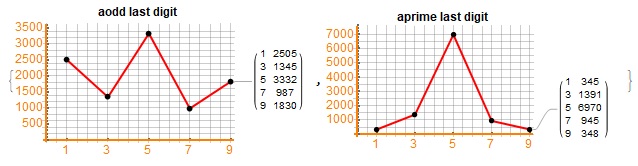
Last Digits and Alt Signal Sum Mod:
Another feature that is worth analyzing is the frequency of the last digits of the terms of the sequences. The last digits of each term in the sequences produce somewhat similar graphics, with a visible predominance of the digit 5 for the "aprime". Below are the result for the first 9999 terms of each sequence:
p = {PlotLabels -> Automatic, ImageSize -> 300, GridLines -> All,
  Ticks -> {{1, 3, 5, 7, 9}, Automatic},
  PlotStyle -> Directive[Red, Thick],
  AxesStyle -> Directive[Thick, Orange, 12],
  Map[PlotLabel -> Style[# <> " last digit", Black, Bold] &, {"aodd",
    "aprime"}],
  Map[Epilog -> {PointSize[0.03], Point[#]} &, {p1, p2}]}; p1 =
 SortBy[Union@Tally@Table[Last@IntegerDigits[aodd[i]], {i, 1, 9999}],
  First]; p2 =
 SortBy[Union@
   Tally@Table[Last@IntegerDigits[aprime[i]], {i, 2, 10000}], First];
{ListLinePlot[Callout@p1, p[[1]], p[[2]], p[[3]], p[[4]], p[[5]],
  p[[6]], p[[7, 1]], p[[8, 1]]],
 ListLinePlot[Callout@p2, p[[1]], p[[2]], p[[3]], p[[4]], p[[5]],
  p[[6]], p[[7, 2]], p[[8, 2]]]}
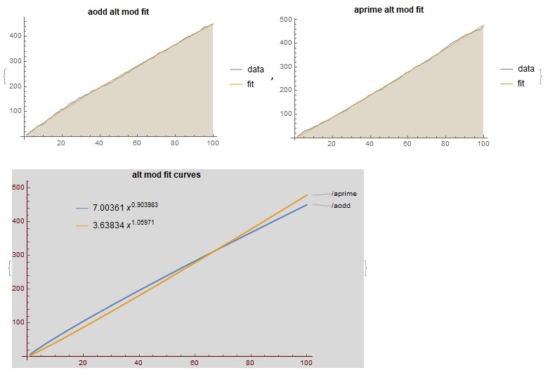
- Alternating Signal Sum Mod:
Although the graphs are a little different for the last digits, analyzing the Mod[_,9], that is, the rest of the division by 9, and then making a “cumulative sum of Mod9 with alternating sign”, we notice that there are a similarity and both are practically linear with model of the type: {a x^b}.
fitmod[n_] :=
 Module[{t, m, f1, f2, m1, m2, u1, u2, v}, Clear[a, b, x];
  t[ty_] :=
   Thread[{Range@n,
     Table[Sum[
       Mod[(-1)^(i)*(ty /. {1 -> aodd, 2 -> aprime})[i], 9], {i, 1,
        j}], {j, 2, n + 1}]}];
  m = a*x^b; f1 = FindFit[t[1], m, {a, b}, x];
  f2 = FindFit[t[2], m, {a, b}, x];
  m1 = Function[{x}, Evaluate[m /. f1]];
  m2 = Function[{x}, Evaluate[m /. f2]];
  u1 = Thread[{Range@n, Table[m1[[2]], {x, 1, n}]}];
  u2 = Thread[{Range@n, Table[m2[[2]], {x, 1, n}]}];
  v = {PlotRange -> All, Filling -> Axis, ImageSize -> 300,
    PlotLegends -> {"data", "fit"},
    PlotStyle -> {Automatic, Thickness[0.004]}};
  Print[{ListLinePlot[{t[1], u1}, v[[1]], v[[2]], v[[3]], v[[4]],
     v[[5]], PlotLabel -> Style["aodd alt mod fit", Black, Bold]],
    ListLinePlot[{t[2], u2}, v[[1]], v[[2]], v[[3]], v[[4]], v[[5]],
     PlotLabel -> Style["aprime alt mod fit", Black, Bold]]},
   {ListLinePlot[{u1, u2}, PlotRange -> All, ImageSize -> 500,
     PlotLegends -> Placed[{m1[[2]], m2[[2]]}, {0.33, 0.8}],
     PlotStyle -> {Thickness[0.005], Thickness[0.005]},
     Background -> LightGray, AxesStyle -> Darker[Red, 0.6],
     PlotLabels -> {"/aodd", "/aprime"},
     PlotLabel -> Style["alt mod fit curves", Black, Bold]]}]]
Below are the results and the fit:
fitmod[100]
Factor Integers and TreePlot:
Finally, one of the most interesting analyzes is that of integer factors. In this type of analysis, the sequence terms are factored and the number of: different factors, total factors and which types of terms are linked by each factor (TreePlot) and are related.
- Factor Integers (Quantification):
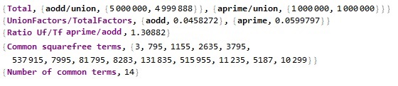
In an extensive analysis, I used 5000000 terms for “aodd” and 1000000 terms for “aprime” (long time to evaluate).
The first striking feature is that some terms are repeated in the “aodd” sequence from time to time (in 5000000 terms, 112 repeated), which does not occur in “aprime” (all 1000000 terms are unique).
The second characteristic is that the ratio between the number of different integer factors divided by the total of integer factors; it is higher for “aprime” (6%), while “aodd” is 4.58%. That is, “aprime” has 30.8% more unique integer factors than “aodd” in this relatively large sampling interval (I know that the samples have different quantities, but the terms are a little bit closer with these numbers and even with a sample of the same size, a higher value for the ratio is still found for "aprime").
Surprisingly, a great peculiarity found is that only 14 terms are the same for the two sequences in this relatively large sample. However, these numbers do not form a true sequence, because if we increase the sample size, a term can be inserted in the middle of these numbers, that is, it is a "sequence" with frequent changes in the positions of the terms.
facInt[o_, p_] :=
 Module[{o2, p2, n1, n2, f1, f2, f3, f4, f5, f6, nn},
  o2 = Table[aodd[i], {i, 1, o}];
  p2 = Table[aprime[i], {i, 1, p}]; {n1, n2} =
   Map[{Length@#, Length@Union@#} &, {o2, p2}]; {f1, f4} =
   Map[Flatten[FactorInteger[#], 1] &, {o2, p2}]; {f2, f5} =
   Map[Length@# &, {f1, f4}]; {f3, f6} =
   Map[Length@Union@# &, {f1, f4}];
  nn = Keys[
    DeleteCases[
     Normal@Counts@Join[Keys@Normal@Counts@o2, p2], _ -> 1]];
  Column[{{Style["Total", Bold, Purple], {Style["aodd/union", Bold],
      n1}, {Style["aprime/union", Bold], n2}}, {Style[
      "UnionFactors/TotalFactors", Bold,
      Purple], {Style["aodd", Bold],
      N[f3/f2]}, {Style["aprime", Bold], N[f6/f5]}}, {Style[
      "Ratio Uf/Tf aprime/aodd", Bold, Purple],
     N[(f6/f5)/(f3/f2)]}, {Style["Common squarefree terms", Bold,
      Purple], nn}, {Style["Number of common terms", Bold, Purple],
     Length@nn}}]]
facInt[5000000, 1000000]
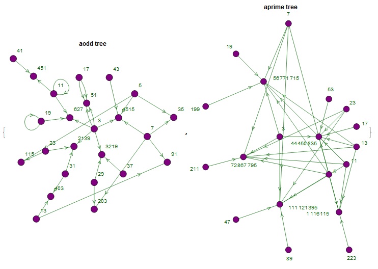
A tool that proves to be important, and mainly not for the visual aspect, but for the ability to analyze the integer factors, was the TreePlot[].
atree[type_, in_ : 1, n_] :=
  Module[{d, a1, a2, a3},
   a1 = Table[
     ToExpression[
      type <> "[i]"], {i, (type /. {"aodd" -> 1,
         "aprime" -> 2}), (type /. {"aodd" -> n,
         "aprime" -> n + 1})}]; d = n - in; a2 = FactorInteger[a1];
   a3 = Flatten@
     Table[Map[# -> a1[[y]] &,
       Table[a2[[y, x]][[1]], {x, 1, Length@a2[[y]]}]], {y, in,
       Length@a1}];
   TreePlot[Map[Tooltip[#] &, a3], Center,
    VertexLabels -> If[d > 25, None, Automatic],
    VertexShapeFunction -> If[d > 45, None, Automatic],
    PlotLabel -> Style[type <> " tree", Black, Bold, Opacity[1]],
    PlotStyle ->
     If[d > 100, Directive[Opacity[0.2], Blue, Thin],
      Directive[Darker[Green, 0.6], Thin]],
    DirectedEdges -> If[d > 80, False, True],
    EdgeShapeFunction ->
     If[d > 100, Automatic,
      GraphElementData["ShortUnfilledArrow", "ArrowSize" -> 0.033]],
    VertexStyle -> Purple, VertexSize -> 0.3, ImageSize -> 350]];
Below are the terms from 5 to 18 for "aodd" and the terms from 16 to 20 (excluding the initial 0) for "aprime", and their integer factors, showing the direct links to their terms:
{atree["aodd", 5, 18], atree["aprime", 16, 20]}
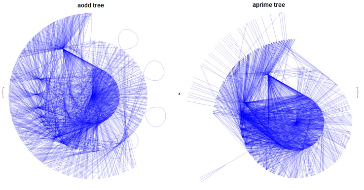
For a better understanding, I was able to visualize the behavior from the first term to the term 500 and 250, for the “aodd” and “aprime”, respectively, with their integer factors linked. In this case, the analysis is visual:
{atree["aodd", 500], atree["aprime", 250]}
Links:
https://oeis.org/A334176
https://oeis.org/A334177
Thanks.


