Message Boards Message Boards

0
|
4183 Views
|
2 Replies
|
1 Total Likes
View groups...
Share
Share this post:

Fitting Data With Poisson and Normal Distributions With Fit Data (Chi^2)

Posted 4 years ago

Hello!

I have been at this for a week and I don't know where else to ask. I am trying to solve for chi^2 from a distribution fit using Mathematica. I have the following data:

{812,827,782,841,839,803,800,818,790,838,783,768,799,854,805,832,786,838,802,805,825,784,797,808,846,809,814,857,884,855,800,855,818,865,801,823,812,861,807,830,813,827,819,796,870,825,827,872,770,849,813,828,839,804,805,833,833,871,856,819,787,819,852,786,864,841,799,804,812,831,830,810,863,856,794,808,794,838,748,757,866,778,823,818,830,794,831,838,853,836,821,836,797,863,811,867,803,821,864,819}

It is expected that this data will follow Poisson and Normal Distributions. I can get these fit parameters by using FindDistributionParameters[]. I can also plot these distribution equations against the data to show that it's a good fit visually speaking (although the units may be incorrect):

Fits vs Data

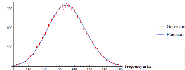
What I can't figure out though is how to obtain data showing why this is a good fit, specifically the value chi^2 (which is required for what I am doing.) I tried to calculate this manually, but my values are way off what my peers are obtaining using different programs. The equation I am attempting to solve manually is this oneL Chi^2 Equation

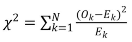
Where Ok is the measured point and Ek is the point as expected by the fit. I don't think this is working because I think this equation requires actual values, while Mathematica's Poisson and Normal distributions are probability based. Here's the code I have been using:

FindDistributionParameters[CS2S1r, NormalDistribution[Mu, Sig]]
FindDistributionParameters[CS2S1r, PoissonDistribution[Mu]]
mu = 822.04;
sig = 27.6452;
binCount= 100;
Chi2g = 0;
Chi2p = 0;
h[x_] = PDF[HistogramDistribution[CS2S2r, binCount], x]
f[x_] = PDF[NormalDistribution[mu, sig], x];
g[x_] = PDF[PoissonDistribution[mu], x];
For[i = 764;, i <= 892, i += 1, Chi2g += (h[i] - f[i])^2/f[i]];
For[i = 764;, i <= 892, i += 1, Chi2p += (h[i] - g[i])^2/g[i]];

Here, mu is the mean of the distribution and sig is the standard deviation. Both of these were determined by using FindDistributionParameters[]. binCount is a number I am going to tweak later, but I set it as high as I could so that each step is the same size as the steps in the data. CS2S2r is the name of my data itself, and 764 and 892 were chosen as the bounds because those are the greatest and smallest numbers found in the data itself.

Does anyone know how I might obtain this? Am I fitting the distributions in the correct way? Is there anything else I should do differently?

All help is appreciated, thank you!

Edit: It looks like FindDistribution[] does what I am looking for, but I am not sure if the ChiSquared that it reports is the actual ChiSquared value, or if it's the p-value that comes from a non displayed ChiSquared. I also don't know how to get this to work with error bars, any ideas?

2 Replies
Posted 4 years ago

I don't know how you constructed that figure so I'm ignoring it.

Mathematica has a command (DistributionFitTest) that should test for any distribution but it either takes too long or doesn't finish for a Poisson when the counts are very high as in your example. So here is a brute force approach.

data = {812, 827, 782, 841, 839, 803, 800, 818, 790, 838, 783, 768, 
   799, 854, 805, 832, 786, 838, 802, 805, 825, 784, 797, 808, 846, 
   809, 814, 857, 884, 855, 800, 855, 818, 865, 801, 823, 812, 861, 
   807, 830, 813, 827, 819, 796, 870, 825, 827, 872, 770, 849, 813, 
   828, 839, 804, 805, 833, 833, 871, 856, 819, 787, 819, 852, 786, 
   864, 841, 799, 804, 812, 831, 830, 810, 863, 856, 794, 808, 794, 
   838, 748, 757, 866, 778, 823, 818, 830, 794, 831, 838, 853, 836, 
   821, 836, 797, 863, 811, 867, 803, 821, 864, 819};

(* Determine bins which would hold approximately equal numbers of 
   observations if the distribution was Poisson *)
dist = PoissonDistribution[Mean[data] // N];
nBins = 12;
bins = Join[{-1}, Table[InverseCDF[dist, i/nBins], {i, nBins - 1}], {\[Infinity]}] // Quiet
(* {-1,783,794,803,810,816,822,828,834,841,850,862,\[Infinity]} *)

(* Observed counts *)
observed = Table[Length[Select[data, bins[[i]] < # <= bins[[i + 1]] &]], {i, nBins}]
(* {7,8,11,10,7,9,8,8,10,2,9,11} *)

(* Expected counts *)
n = Length[data];
expected = Table[n (CDF[dist, bins[[i + 1]]] - CDF[dist, bins[[i]]]) // N, {i, nBins}]
(* {8.86592, 7.98339, 9.1535, 8.54294, 8.01289, 8.31321, 8.25561, 
7.84997, 8.25645, 8.72493, 8.04893, 7.99226} *)

(* Chisquare statistic *)
chisq = Total[(observed - expected)^2/expected]
(* 8.00515 *)

(* P-value *)
pValue = 1 - CDF[ChiSquareDistribution[nBins - 2], chisq]
(* 0.628334 *)
POSTED BY: Jim Baldwin

This was really helpful, I appreciate this a whole lot! I even learned new tricks Mathematica can do that I wasn't aware of (such as // N). I also didn't know that pValue was calculated from a ChiSquareDistribution.

The only part I don't understand fully is what exactly is going on in the first portion. I would like to construct a similar system of equations for the Gaussian and possibly a Binomial portion, and I believe this is the part I would change (in addition to the bin number at the very end), but I don't quite get how this determines equally sized bins. Do you run the equation multiple times, changing the value for nBins, until you get an array of numbers in which are all integers? And finally, why do you append a -1 and infinity at the beginning and the end of this array?

Thank you so much, I've learned more from this post than anything I've tried in the past 48 hours trying to get this to work!

Reply to this discussion
Community posts can be styled and formatted using the Markdown syntax.
Reply Preview
Attachments
Remove
or Discard

Group Abstract Group Abstract