Message Boards Message Boards

3D Helmholtz resonance in the violin body with f-holes

Wolfram notebook is attached at the end of the post.


enter image description here

This post is about FEM simulation of violin vibration modes in 3D. As well known there are Helmholtz resonances of air inside the violin body with frequencies dependent on geometry of f-holes. This is the main reason why violin has so pronounced sound. To simulate these modes with Mathematica FEM we first define the body geometry (this is my design with given volume and area of f-holes, but it taken from the real violin):

xy = {{3.805405405405406`,3.34954954954955`},{3.8252252252252257`,6.6990990990991`},{3.9441441441441443`,7.9081081081081095`},
{4.47927927927928`,8.601801801801802`},{5.014414414414414`,8.264864864864865`},{4.816216216216216`,7.8882882882882885`},
{4.895495495495496`,7.630630630630631`},{5.232432432432433`,7.432432432432433`},{5.47027027027027`,7.491891891891892`},
{5.648648648648649`,7.8882882882882885`},{5.668468468468468`,8.046846846846847`},{5.56936936936937`,8.403603603603605`},
{5.252252252252252`,8.681081081081082`},{4.855855855855856`,8.780180180180182`},{4.518918918918919`,8.8`},
{3.9639639639639643`,8.522522522522523`},{3.567567567567568`,7.967567567567568`},{3.3693693693693696`,7.372972972972973`},
{3.2306306306306305`,6.67927927927928`},{3.1513513513513516`,3.3693693693693696`},{3.1513513513513516`,2.655855855855856`},
{2.9729729729729732`,1.783783783783784`},{2.8738738738738743`,1.4666666666666668`},{2.100900900900901`,0.7927927927927928`},
{1.7243243243243245`,1.3081081081081083`},{2.021621621621622`,1.7639639639639642`},{2.0414414414414415`,2.0414414414414415`},
{1.9621621621621623`,2.23963963963964`},{1.6648648648648652`,2.4378378378378383`},{1.4666666666666668`,2.5171171171171176`},
{1.10990990990991`,2.338738738738739`},{0.891891891891892`,1.9423423423423425`},{0.9315315315315316`,1.4072072072072073`},
{1.5657657657657658`,0.7927927927927928`},{2.081081081081081`,0.6342342342342343`},{2.5963963963963965`,0.7927927927927928`},
{3.0918918918918923`,1.2090090090090093`},{3.5081081081081082`,1.902702702702703`},{3.706306306306306`,2.6954954954954955`}};

reg1 = RegionUnion[Disk[{0, 19.5/2}, 19.5/2], 
  Disk[{0, 36 - 15.5/2}, 15.5/2], 
  Rectangle[{-10, 15}, {10, 25}]]; reg2 = 
 RegionDifference[reg1, 
  RegionUnion[Disk[{-10, 20}, 9.5/2], Disk[{10, 20}, 9.5/2]]];
c0 = {0, 36 - 15.5/2}; c1 = {7.03562, 25}; 
f[x_] := c0[[2]] + x (c1[[2]] - c0[[2]])/(c1[[1]] - c0[[1]]); r1 = 
 Norm[c1 - {10, f[10]}];
reg3 = RegionDifference[reg2, Disk[{10, f[10]}, r1]]; 
f1[x_] := c0[[2]] - x (c1[[2]] - c0[[2]])/(c1[[1]] - c0[[1]]);
reg4 = RegionDifference[reg3, Disk[{-10, f1[-10]}, r1]]; c10 = {0, 
  19.5/2}; c11 = {8.215838362577491`, 15}; 
f11[x_] := c10[[2]] + x (c11[[2]] - c10[[2]])/(c11[[1]] - c10[[1]]);
r2 = Norm[c11 - {10, f11[10]}];
reg5 = RegionDifference[reg4, Disk[{10, f11[10]}, r2]]; 
f12[x_] := c10[[2]] - x (c11[[2]] - c10[[2]])/(c11[[1]] - c10[[1]]);
reg6 = RegionDifference[reg5, Disk[{-10, f12[-10]}, r2]]; p6 = 
 RegionPlot[reg6, AspectRatio -> Automatic];
fh[xf_, yf_] := 
  RegionUnion[
   Polygon[Table[{xy[[i, 1]] - xf, xy[[i, 2]] + yf}, {i, 
      Length[xy]}]], 
   Polygon[Table[{-xy[[i, 1]] + xf, xy[[i, 2]] + yf}, {i, 
      Length[xy]}]]];

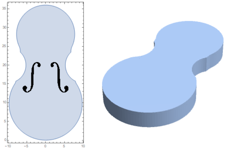
General view of the violin body from the front and back side

Show[p6, Graphics[fh[7, 12], AspectRatio -> Automatic]] 
dz = 3.79; reg8 = 
 ImplicitRegion[Element[{x, y}, reg6] && 0 <= z <= dz, {x, y, z}];
mesh3d1 = DiscretizeRegion[reg8, {{-10, 10}, {0, 36}, {0, dz}}]

Figure 1
Next step is the computation of air modes in the violin body with using NDEigensystem[] as follows

ca = 34321(*T=20C*); L = -Laplacian[u[x, y, z], {x, y, z}]; {vals, funs} = 
NDEigensystem[{L, 
DirichletCondition[u[x, y, z] == 0, 
Element[{x, y}, fh[7, 11.49]] && z == dz]}, u, 
Element[{x, y, z}, mesh3d1], 15];

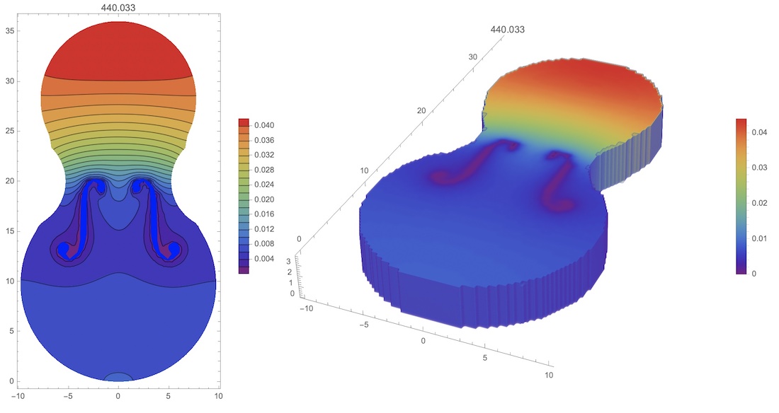
Finally we visualize first 5 modes and the main mode in 3D

{Table[DensityPlot[funs[[i]][x, y, dz/2], {x, -10, 10}, {y, 0, 36}, 
  PlotRange -> All, PlotLabel -> ca Sqrt[vals[[i]]]/(2 Pi), 
  ColorFunction -> "Rainbow", AspectRatio -> Automatic], {i, 1, 
  5}],
 DensityPlot3D[
 funs[[1]][x, y, z], {x, -10, 10}, {y, 0, 36}, {z, 0, dz}, 
 PlotRange -> All, PlotLabel -> ca Sqrt[vals[[1]]]/(2 Pi), 
 ColorFunction -> "Rainbow", AspectRatio -> Automatic, 
 PlotLegends -> Automatic, PlotPoints -> 100, BoxRatios -> Automatic, 
 OpacityFunction -> None, Boxed -> False]} 

Figure 2 
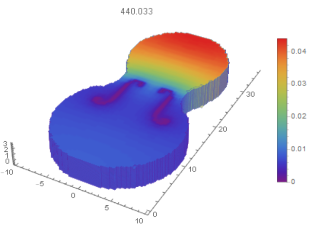
Therefore the first mode of 440.033 Hz is close to "A4" (440 Hz) tone. But we expecting "C4" (261.626 Hz), or "C#4" (277.183 Hz). The main reason of this discrepancies could be the wood plate vibration from the back side. Thus we define mesh, parameters of the wood plate and modes as follows

dreg = DiscretizeRegion[reg6, {{-10, 10}, {0, 36}}, 
  MaxCellMeasure -> .05]
Y = 10.8*10^9; nu = 31/100; rho = 500; h = .003; d = 
 10^4 Sqrt[Y h^2/(12 rho (1 - nu^2))];Ld2 = {Laplacian[-d u[x, y], {x, y}] + 
    v[x, y], -d Laplacian[v[x, y], {x, y}]};

{vals, funs} = 
  NDEigensystem[{Ld2, DirichletCondition[u[x, y] == 0, True]}, {u, v},
    Element[{x, y}, dreg], 5];

Table[DensityPlot[Re[funs[[i, 1]][x, y]], {x, y} \[Element] dreg, 
  PlotRange -> All, PlotLabel -> vals[[i]]/(2 Pi), 
  ColorFunction -> "Rainbow", AspectRatio -> Automatic], {i, 2, 
  Length[vals]}]

Figure 3 
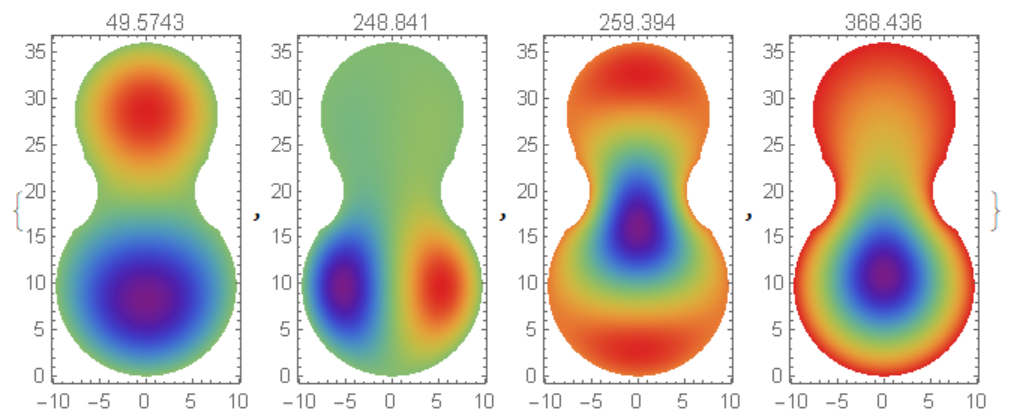
Hence for wood plate we have mode of 259.394 Hz and it is close to C4 tone.

Attachments:
19 Replies
Posted 3 years ago

What about the curvature of the top and back, how do you simulate that?

POSTED BY: Ser Man

It is not so difficult problem for FEM implementations. Please, see my post on https://mathematica.stackexchange.com/questions/214279/3d-elastic-waves-in-a-glass

Posted 3 years ago

You should consider air effects also. If I build a violin which is very low and flat, it makes nasal and very superficial sound. If I build a violin with concave surfaces, it tends to generate more resonance, even if the wood is very young and thus vibrates less that older wood. So the effect from the size and shape of the acoustic chamber is very important, which comes from the circulating air waves.

POSTED BY: Ser Man

Thank you very much for your professional remarks. Actually there are 3D air modes coupled with 2D plate vibration in our model. Also it is possible to simulate effect of plate curvature on the frequency.

Congratulations! Your post was highlighted on the Wolfram's official social media channels. Thank you for your contribution. We are looking forward to your future posts.

POSTED BY: Moderation Team
Posted 3 years ago

Hi Alexander,

Sorry for the later reply. I think you made a good approach for coupling air and wood. However, DirichletCondition is probably too strong in this case, all frequencies come from the wood, no air effect at all.

I proposed to solve NDEigensystem in one shot.

(* material parameters for bottom solid wood region *)
Y = 10.8*10^9;
nu = 31/100;
rho = 500;
h = .003;
d = 10^4 Sqrt[Y h^2/(12 rho (1 - nu^2))];

(* material parameters for upper fluid air region *)
ca = 34321  (* Need to check air parameters, Is it right for this \
equation ??? f=ca^2 vals\[LeftDoubleBracket]i\[RightDoubleBracket]/(2 \
Pi)^2 *);  

(* coupled coeffiency based on Z position *)
 cp = If[z == 0, d, ca];

(* governing equations *)
Ld3 = {Laplacian[-cp u[x, y, z], {x, y, z}] + 
    v[x, y, z], -cp  Laplacian[v[x, y, z], {x, y, z}]};

{vals, funs} = 
  NDEigensystem[{Ld3, 
    DirichletCondition[u[x, y, z] == 0, 
     Element[{x, y}, fh[7, 11.49]] && z == dz]}, {u, v}, 
   Element[{x, y, z}, mesh3d1], 16];

plot = Grid@
  Partition[
   Table[ContourPlot[
     funs[[i, 1]][x, y, dz - .1], {x, -10, 10}, {y, 0, 36}, 
     PlotRange -> All, PlotLabel -> vals[[i]]/(2 Pi), 
     ColorFunction -> "Rainbow", AspectRatio -> Automatic, 
     PlotLegends -> Automatic, PlotPoints -> 80, Contours -> 20], {i, 
     2, Length[vals]}], UpTo[5]]

enter image description here I don't think, this result is numerical right at the moment, because air parameter "ca" seems almost same quantity level as wood parameter “d". The above code is just show you the possibility to combine two subjects (wood and air) in one equation and solve it together.

POSTED BY: Frederick Wu

Thank you very much for your answer. It seems to me that extinction of 2D elastic model to 3D acoustic model has no physical background.

Posted 3 years ago

Usually, the acoustic wave equation describes sound waves in a liquid or gas. I am not sure if it is capable to works in solid as well. Anyway, If it agrees with your experiment, we accept it.

I suggest you can approach a coupled eigenvalue modal with both wooden and air with a few steps.

  1. Firstly, couple that solid wooden wave equation with air acoustic wave equation, since they are both in Laplacian-form now. Maybe define one united equation works both for wood and air. Maybe it's looks like a piecewise funtion.
  2. Then, define two kinds of regions (air and solid material property) with coupled/merged boundary meshes, but regard it as one-piece of mesh in solver.
  3. Finally, feed NDEigensystem with one united wave equation and one coupled mesh region to calculate a coupled eigenvalue for frequency.

Still, define the governing equation and boundary will be a headache thing.

Wolfram Documentation two examples might be helpful. PDEModels/tutorial/Acoustics/ModelCollection/AcousticCloak PDEModels/tutorial/Acoustics/ModelCollection/RoomEigenfrequencies

POSTED BY: Frederick Wu

Please, look attentively on equations used to calculate bending mode in a wooden plate. It is derived from well known equation commonly used for plates and beams as follows $$\rho h u_{tt}+D \nabla ^4 u=0$$ The one possible way to compute air modes in the body generated by back plate is DirichletCondition[] for the 3D wave equation. Note that the wave equation turns to the Helmholtz equation since we are search the mode generated by the plate vibration. Code to calculate plate modes (we use dreg from above)

Y = 10.8*10^9; nu = 31/100; rho = 500; h = .003; d = 
 10^4 Sqrt[
   Y h^2/(12 rho (1 - nu^2))]; Ld2 = {Laplacian[-d u[x, y], {x, y}] + 
   v[x, y], -d Laplacian[v[x, y], {x, y}]};
{vals, funs} = 
  NDEigensystem[{Ld2, DirichletCondition[u[x, y] == 0, True]}, {u, v},
    Element[{x, y}, dreg], 10, 
   Method -> {"Interpolation" -> {"ExtrapolationHandler" -> \
{Automatic, "WarningMessage" -> False}}}];
Table[DensityPlot[Re[funs[[i, 1]][x, y]], {x, y} \[Element] dreg, 
  PlotRange -> All, PlotLabel -> vals[[i]]/(2 Pi), 
  ColorFunction -> "Rainbow", AspectRatio -> Automatic], {i, 2, 
  Length[vals]}]

Figure 1
Code to compute modes in the body with f-holes (we use mesh1=mesh3d1 and ca from the code above)

Do[solp[i] = 
   NDSolveValue[{-u[x, y, z] (vals[[i]]/ca)^2 - 
       Laplacian[u[x, y, z], {x, y, z}] == 0, 
     DirichletCondition[u[x, y, z] == Re[funs[[i, 1]][x, y]], z == 0],
      DirichletCondition[u[x, y, z] == 0, 
      Element[{x, y}, fh[7, 11.49]] && z == dz]}, u, 
    Element[{x, y, z}, mesh1]];, {i, 2, Length[vals]}]

Table[Show[
  ContourPlot[solp[i][x, y, dz - .1], {x, -10, 10}, {y, 0, 36}, 
   PlotRange -> All, ColorFunction -> "Rainbow", 
   AspectRatio -> Automatic, PlotLegends -> Automatic, 
   PlotPoints -> 50, Contours -> 20, PlotLabel -> vals[[i]]/(2 Pi)], 
  Graphics[{Green, 
    Polygon[Table[{xy[[i, 1]] - 7, xy[[i, 2]] + 11.49}, {i, 
       Length[xy]}]], 
    Polygon[Table[{-xy[[i, 1]] + 7, xy[[i, 2]] + 11.49}, {i, 
       Length[xy]}]]}]], {i, 2, Length[vals]}]

Figure 2

Posted 3 years ago

Hi Alexander,

One question, where you got the below equations to calculate eigenvalue for solid wood plane?

d = 10^4 Sqrt[Y h^2/(12 rho (1 - nu^2))]; 
Ld2 = {Laplacian[-d u[x, y], {x, y}] + v[x, y], -d Laplacian[v[x, y], {x, y}]};;

I am confused by Wolfram documentation ( NDEigensystem > application > structure ). They recommend a plane stress to calculate eigenvalue for solid plane, instead of using Laplacian? Which one is correct for solid? Plane stress or Laplacian operator? What is your opinion?

https://reference.wolfram.com/language/ref/NDEigensystem.html

POSTED BY: Frederick Wu

As it well known the wood is anisotropic material. Also we are looking for bending waves in a wooden plate with a very special design. Therefore we can state that this kind of waves could be described with 3D elastic model for anisotropic material or with 2D model for the wooden plate. After some numerical experiments I have decided that there is one 2D model with desired frequencies.

Posted 3 years ago

I found below information for you. John Coffey's paper with FEA is highly recommended. He proposed a coupled oscillations of two masses and springs model to analysis wood effect on frequency.

In short, A lot of works with air dynamic, acoustic, mechanical vibration. In my opinion, It's better to start from ideal Helmholtz resonator, then circle-hole guitar, then f-holes violin. Violin is the hardest Helmholtz resonator project.

Hopefully, It helps for your project.

https://newt.phys.unsw.edu.au/jw/Helmholtz.html

https://www.lisafea.com/pdf/JMC-HelmholtzResonance--Rb-shorter.pdf

POSTED BY: Updating Name

Thank you for the link to the paper The Air Cavity, f -holes and Helmholtz Resonance of a Violin or Viola by John Coffey. Note, while we have very similar design with volume of 2 liters and similar f-holes, the main mode very differ in two cases: 312 Hz as reported by John Coffey and 440 Hz as shown above.

Posted 3 years ago

Hi Alexander,

  1. I think you add Dirichlet Condition, that make f-holes on contours. So, each mode has f-holes contours more or less.

    DirichletCondition[u[x, y, z] == 0, Element[{x, y}, fh[7, 11.49]] && z == dz]
    

enter image description here

  1. Calculating only 2D back plate might not sufficient to view all solid modes on violin. so I suggest a 3D shell region violin might helps. enter image description here enter image description here enter image description here

  2. Real violin inner structure can be more complex, "Bass bar" and "sound post" may also affect. enter image description here

I attached your notebook, I worked for a little.

Attachments:
POSTED BY: Frederick Wu

Thank you very much for your advanced code. Your 3D mesh better then that I am used. Also we have this question. How we can connect back plate modes with Helmholtz resonance?

Thank you very much for your post. While playing around with the code, I came upon what looks like a bug in DiscretizeRegion:

RegionPlot[RegionBoundary@reg6]
RegionPlot[DiscretizeRegion@RegionBoundary@reg6, PlotRange -> All]
POSTED BY: Gianluca Gorni
Posted 3 years ago

Hi Alexander,

Excellent Finding, Congratulations!

I have one question, how can we explain the performance f-holes from viewpoint of acoustics? Opening f-hole is the best solution to minimum negative effect at 1 mode (440 Hz) for ideal air resonator? It seems the shape or boundary of violin determinate the f-holes on contours ? What is your opinion?

You may interest to read this paper. https://dspace.mit.edu/handle/1721.1/61924

POSTED BY: Updating Name

Thank you for link to the thesis page Acoustic Function of Sound Hole Design in Musical Instruments by Hadi Tavakoli Nia. Also I would like to path to this page by Martin Schleske. With my code we can compute some modes of air vibration in the violin body and back plate vibration. Your question about performance of f-holes is very professional and we are even not supposed to answer it on this forum about Mathematica. Briefly we can say only that you are right about shape of boundary and f-holes. With this code we can calculate how the main frequency depends on f-holes geometry and position.

enter image description here -- you have earned Featured Contributor Badge enter image description here Your exceptional post has been selected for our editorial column Staff Picks http://wolfr.am/StaffPicks and Your Profile is now distinguished by a Featured Contributor Badge and is displayed on the Featured Contributor Board. Thank you!

POSTED BY: Moderation Team
Reply to this discussion
Community posts can be styled and formatted using the Markdown syntax.
Reply Preview
Attachments
Remove
or Discard

Group Abstract Group Abstract