MODERATORS' NOTE: related resource function is available here.
Schmidt Arrangements
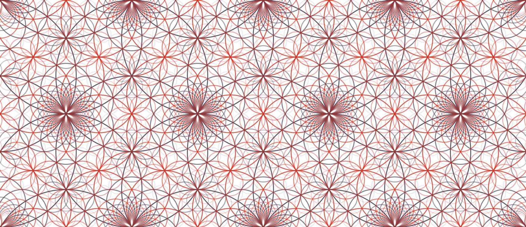
The beautiful picture above is a Schmidt Arrangement : the orbit of R under a specific group of Mobius transformations.
The Mobius transformation of a complex z is f(z)=(az+b)/(cz+d)
If the coefficients a,b,c and d are restricted to the integers of a complex quadratic field then we get a Schmidt Arrangement.
To each circle of a Schmidt Arrangement, you can associate a center c, curvature b, and co-curvature b' (curvature of the circle you get with an inversion).
A circle is part of the Schmidt Arrangement if b b'==c conjugate(c) -1
Said differently, if (c conjugate(c) -1) / b is a multiple of Sqrt(d) where Sqrt(d) is used to generate the quadratic field.
The algorithm is iterating on curvature (up to a max) and on position (between some bounds) and checking if the above divisibility condition is true. If it is, the circle is part of the arrangement.
For more details, download the attached Notebook because I can't write maths here.
Schmidt Arrangements were studied by Kate Stange and Daniel E. Martin and a Sage notebook implementation can be found on their websites:
https://math.katestange.net/illustration/
http://math.colorado.edu/~dama4729/
I have tried to implement a function simple to use for generating a few Schmidt Arrangements. All bugs are mine and not from the original authors. For the known limitations, please download the notebook.
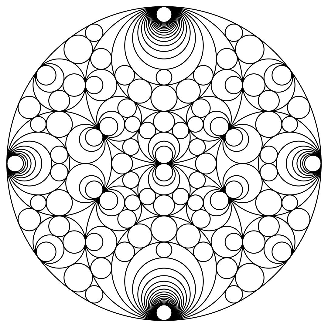
The simplest way to start :
schmidtArrangements[-1]
and you'll get:
There is an option to control the color:
schmidtArrangements[-1, "color" -> {"colourpool", {1, 0}}]
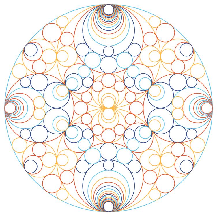
The function is providing some palette and a color function which is using the curvature and some scaling. The list {a,b} (here 1,0) are the scaling factors.
The color index is given by (c * a + b) mod n
n is the number of colors in the palette. c is the curvature of the circle expressed as an integer.
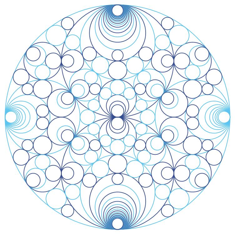
You can force a different n if it is smaller than the palette length. Let's use 2 instead of 4. It is the first value of the list when the list has 3 elements:
schmidtArrangements[-1, "color" -> {"colourpool", {2, 1, 0}}]
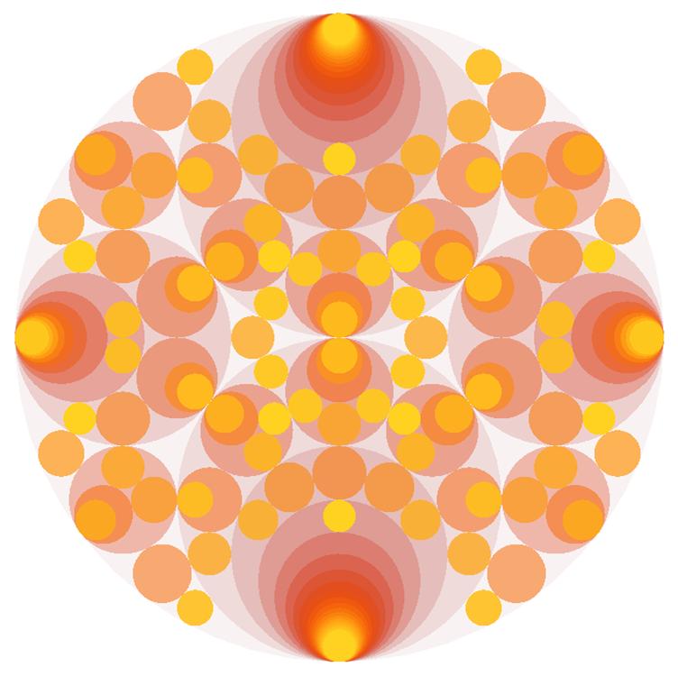
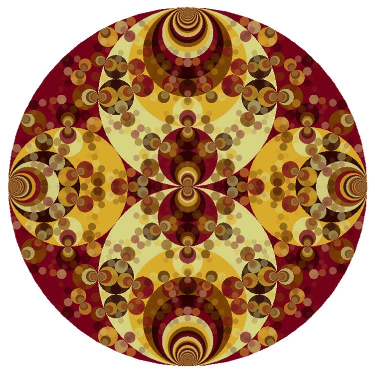
We can also use a standard palette using ColorData. Currently only gradient. The value will be 1 for the max curvature used to compute the picture. The circle can be replaced by disks. And the transparency can increase or decrease with the curvature:
schmidtArrangements[-1, "circle" -> False,  "color" -> ColorData["SolarColors"], Background -> White,
 "transparency" -> "decreasing"]
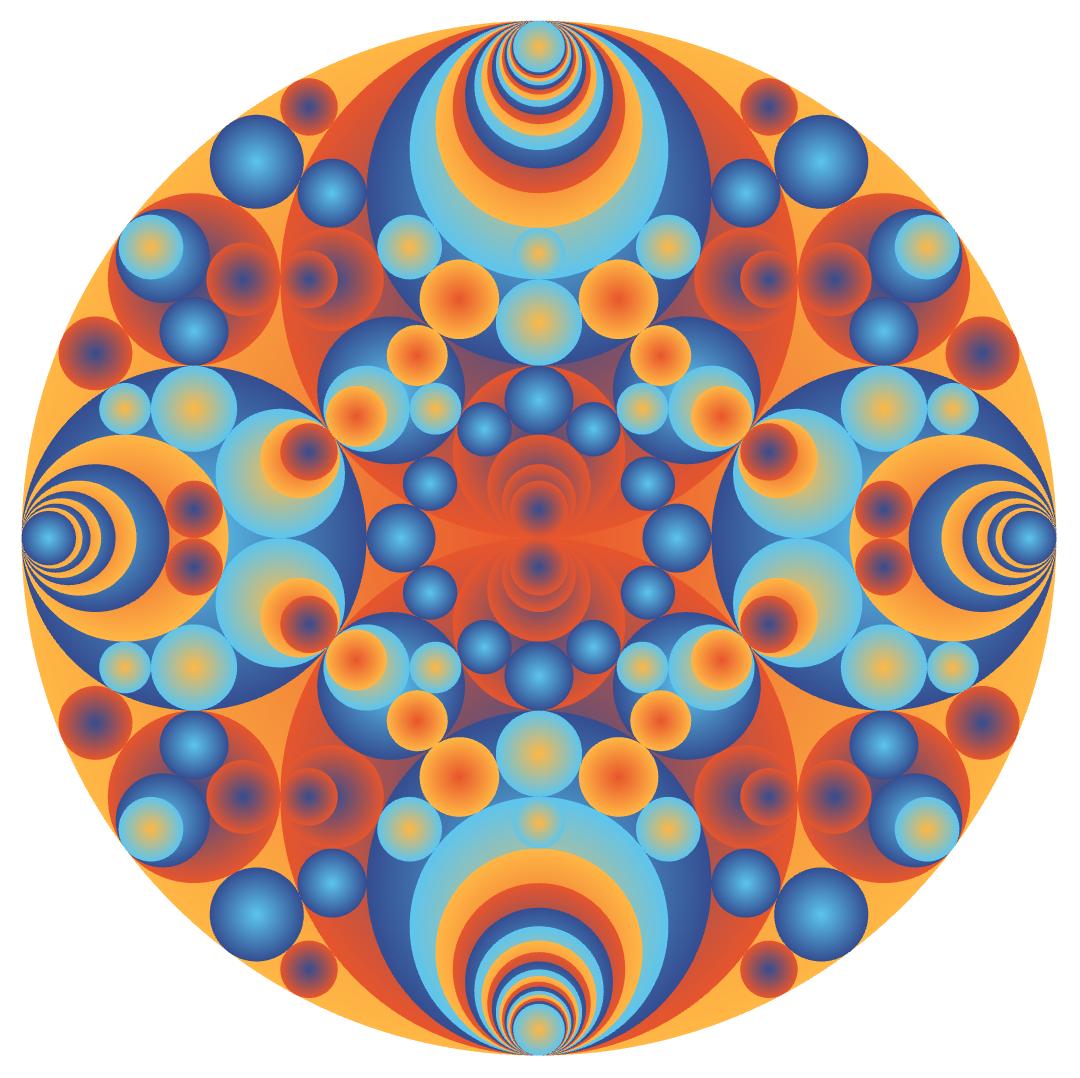
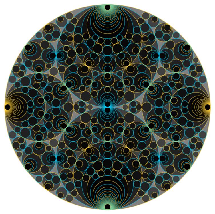
It is also possible to use a Radial gradient:
schmidtArrangements[-1, "circle" -> False,
 "color" -> {"gradient", {"colourpool", {1, 2}}, {"colourpool", {1, 1}}}]
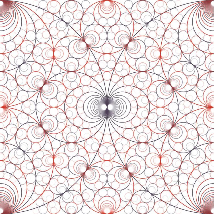
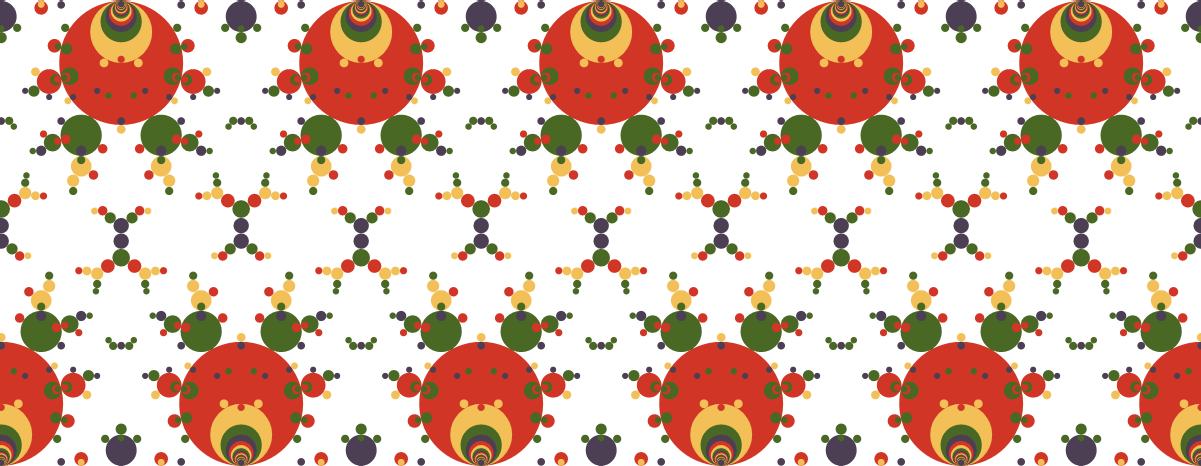
By default, we keep only a Circle in the plane to display the picture. But we can also restrict to a plane. The option "filter" is used for this. Below example is also showing the option "cmax" for the maximum curvature to test.
schmidtArrangements[-1, "cmax" -> 40,
 "color" -> {"coloursaul", {2, 1, 1}},  "transparency" -> "increasing",
 "filter" -> Rectangle[{-0.1, -0.1}, {1.1, 1.1}], PlotRange -> {{0, 1}, {0, 1}}]
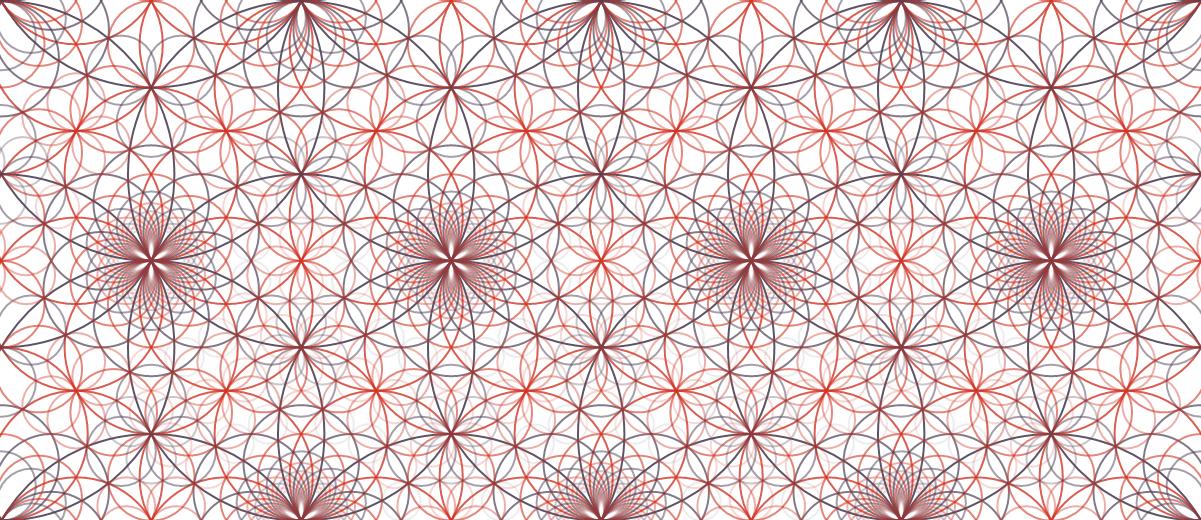
The function is supporting same options as Graphics. In below picture, the root is different (-2) and the background is black:
schmidtArrangements[-2, "cmax" -> 40,  "color" -> {"coloursaul", {2, 1, 1}},
 "transparency" -> "increasing",  "filter" -> Rectangle[{-0.1, -0.1}, {1.1, Sqrt[2.0] + 0.1}],
 PlotRange -> {{0, 1}, {0, Sqrt[2.0]}}, Background -> Black]

Now, let' s play with - 3.
schmidtArrangements[-3, "cmin" -> 0, "cmax" -> 10,  "color" -> {"coloursaul", {2, 1, 1}},
 "transparency" -> "increasing",  "filter" -> Rectangle[{-2.1, -Sqrt[3.0] - 0.1}, {2.1, 2*Sqrt[3.0] + 0.1}],
 PlotRange -> {{-2, 2}, {0, Sqrt[3.0]}}, ImageSize -> Large]
The following example will take more time to compute the result because it is scanning a bigger region of the plane to detect circles member of the Schmidt Arrangement. It is specified with the option "xmax" and "ymax" which in addition to "cmax" are controlling where the search for new circles is taking place.
schmidtArrangements[-15, "cmin" -> 0, "cmax" -> 20,  "color" -> {"coloursaul", {1, 0}}, "xmax" -> 10.0, "ymax" -> 2.0,
 "filter" -> Rectangle[{-0.1, -0.1}, {5.1, Sqrt[15.0] + 0.1}], "circle" -> False, PlotRange -> {{0, 5}, {0, Sqrt[15.0]/2.0}},
 ImageSize -> Large]
When a function is taking time, it is useful to be able to dissociate the part searching for the circles (long) and the styling part (quick). Because generally we'd like to be able to experiment with styling and regenerate different pictures.
The option "precompute" is used for this.
Note that option "cmax" is reused in the display part (with an additional "cmin"). The display part is filtering the circles and displaying only the one which are in a given geometric area and between two curvature boundaries.
For the color palettes, it is this other "cmax" which is used.
Separating the computation from the styling is allowing to use a different "cmax" for both.
In the example below we remove circle which are contained in another circle. It is the option "containment".
precomputed = schmidtArrangements[-1, "cmax" -> 100, "precompute" -> True];

schmidtArrangements[precomputed, "circle" -> False, "containment" -> False, "cmin" -> 2,
"cmax" -> 100,  "color" -> {"colour24", {1, 4}}]
Another long example because the cmax is quite high.
precomputed2 =
  schmidtArrangements[-1, "cmax" -> 100, "precompute" -> True];

schmidtArrangements[precomputed2, "circle" -> False,
 "color" -> {"colour92", {0, 0}}, "transparency" -> 0.5, "cmin" -> 2, "cmax" -> 100]
Since we have precomputed the circles, now we can quickly regenerate a new picture with a different styling.
schmidtArrangements[precomputed2, "circle" -> False,
 "color" -> {"coloura", {0, 0}}, "transparency" -> 0.5, "cmin" -> 2, "cmax" -> 100]
schmidtArrangements[precomputed2, "circle" -> False,   "color" -> {"colour5", {1, 0}},
 "transparency" -> "increasing", "cmin" -> 0, "cmax" -> 75,  "filter" -> Circle[{0., 0.5}, Sqrt[0.25]]]
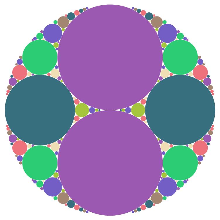
We can also overlay two pictures generated with different styling from the same computation.
Show[
 schmidtArrangements[precomputed2, "circle" -> False, "color" -> Black,
  "transparency" -> 0.5, "cmin" -> 0, "cmax" -> 35, "filter" -> Circle[{0., 0.5}, Sqrt[0.25]]],
 schmidtArrangements[precomputed2,  "color" -> {"colournightlife", {2, 0}},
  "transparency" -> 0.5, "cmin" -> 0, "cmax" -> 35,  "filter" -> Circle[{0., 0.5}, Sqrt[0.25]]]
 ]
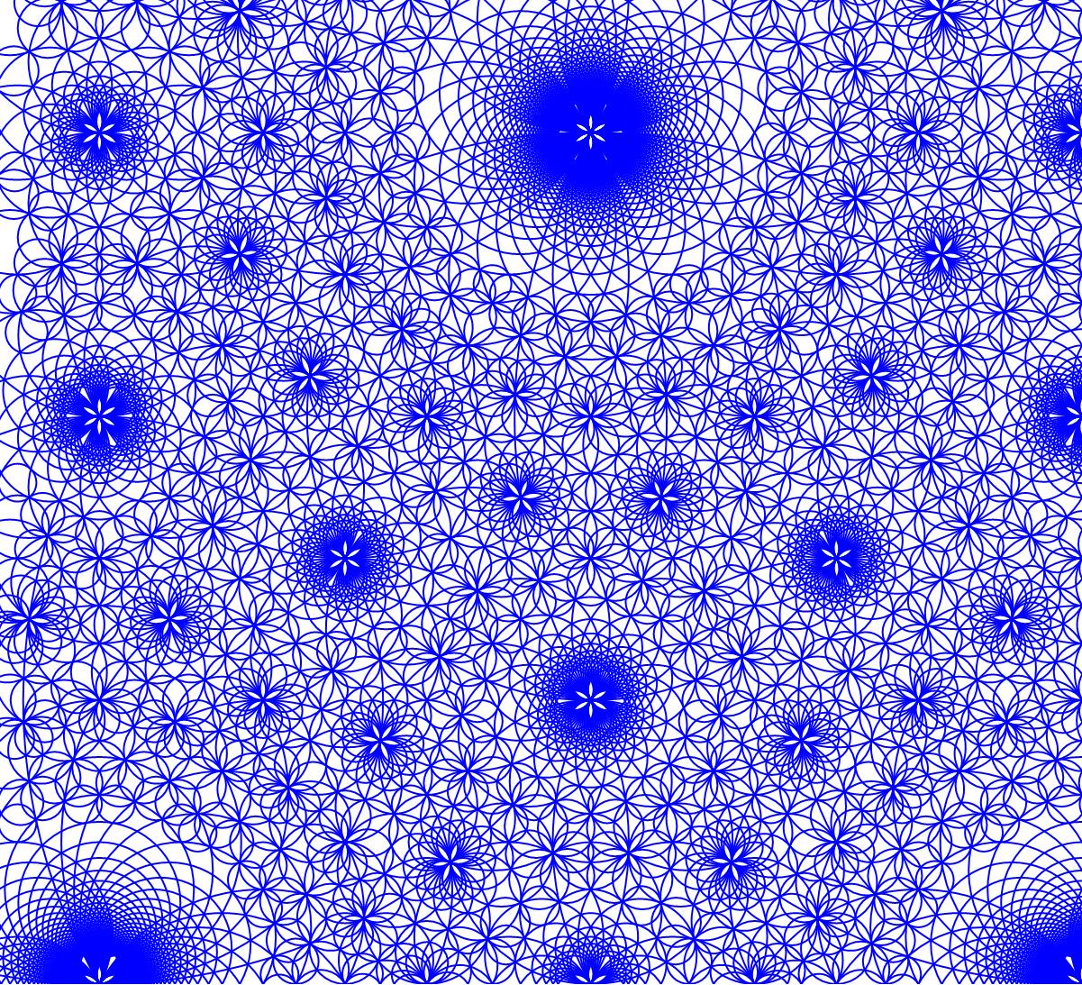
Another example with - 3
schmidtArrangements[-3, "cmin" -> 0, "cmax" -> 30, "color" -> Blue,
 "filter" -> Rectangle[{-0.1, -0.1}, {1.1, 1.1}],
 PlotRange -> {{-0.1, 1}, {0, 1.0}}, ImageSize -> Large]
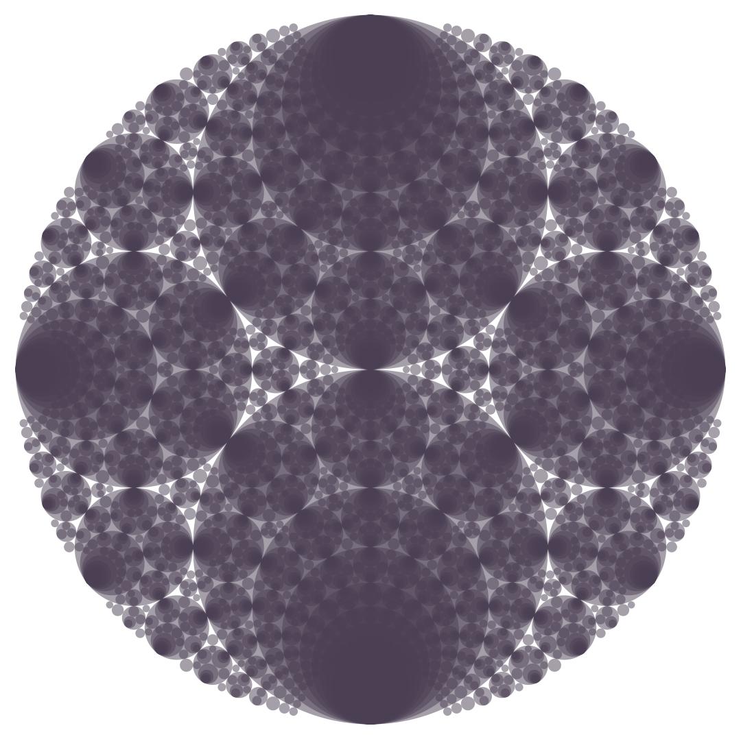
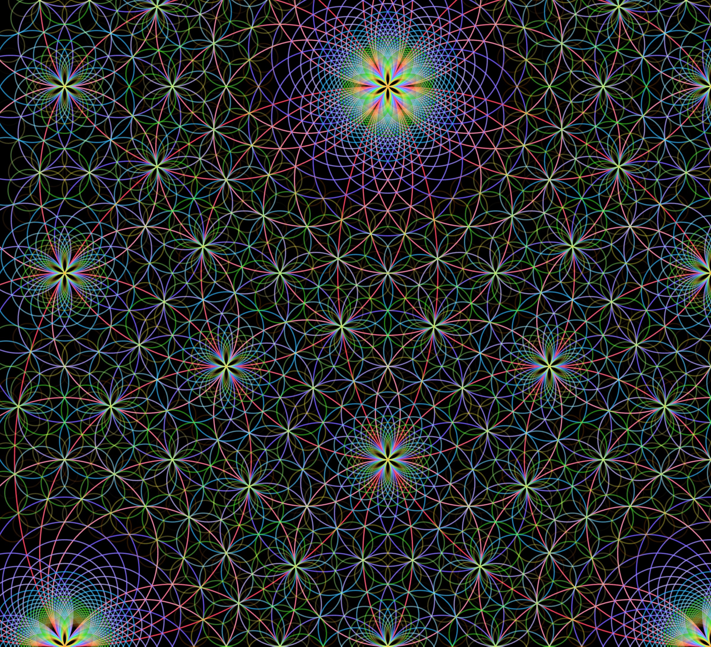
The same example but with a bigger value of cmax.
pre = schmidtArrangements[-3, "cmax" -> 100, "precompute" -> True];
Now you can play with different palettes and filter with different cmax values.
Manipulate[
 schmidtArrangements[pre, "cmin" -> 0, "cmax" -> nb,
  "color" -> ColorData[s], "transparency" -> "increasing",
  "filter" -> Rectangle[{-0.1, -0.1}, {1.1, 1.1}],
  PlotRange -> {{-0.1, 1}, {0, 1.0}}, ImageSize -> Large,
  Background -> Black],
 {s, ColorData["Gradients"]}, {{nb, 30}, {10, 20, 30, 40}}
 ]
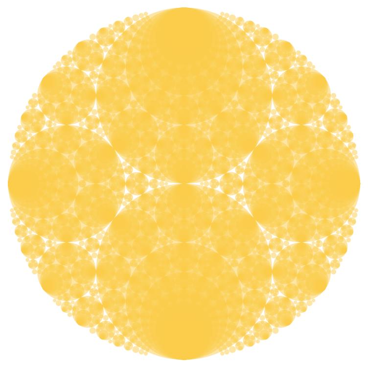
A nice final example :
img = schmidtArrangements[pre, "cmin" -> 0, "cmax" -> 30,
  "color" -> ColorData["BrightBands"], "transparency" -> "increasing",
  "filter" -> Rectangle[{-0.1, -0.1}, {1.1, 1.1}],
  PlotRange -> {{-0.1, 1}, {0, 1.0}}, ImageSize -> Large,
  Background -> Black]
 Attachments:


