Message Boards Message Boards

Generate a shape that contains 95% of my data

Hello all,

I am trying to visualize and compare properties of data from an experiment. This experiment could be anything where a large number of specimens is sampled, resulting in a set of properties from each specimen. I want to compare different conditions (visually) without making a model or any assumptions about the distribution. E.g. this could be anything from nature, e.g. comparing the properties "height" and "number of branches" of different tree species, for each species a few hundred trees.

When drawing the points for the trees in a 2D diagram, one can see that each species covers a certain area of the diagram. I would like to draw some shape into my plot (one for each species) that contains 95% (or any other fraction) of the points. But since my points will not be normally distributed, some other shape than an ellipsoid is needed. Obviously, these data could also have a bi- or multimodal distribution, in which case this shape would split into two or more parts. Also, I would like to do this for 3D (more dimensions are probably useful too but hard to visualize).

Here is a hand-drawn example.

Diagram

Any suggestions how I can achieve this?

Thanks for your ideas,

Max

5 Replies
Posted 3 years ago

Glad it works. And as I'm sure you already know, the "smoothness" of the enclosing shapes is "in the eye of the beholder." Some tweaking of the bandwidths might still be in order but at least you'd still have the 95% of the points encompassed.

POSTED BY: Jim Baldwin

Hello Jim,

great, thanks for this! This is what I was looking for. It works for the 3D case too (looks much cooler in 3D).

dist1 = MixtureDistribution[{1, 
    1}, {MultinormalDistribution[{0.3, 0.5, 
      0.4}, {{0.01, 0, 0}, {0, 0.02, 0}, {0, 0, 0.01}}], 
    MultinormalDistribution[{0.7, 0.6, 
      0.5}, {{0.01, 0, 0}, {0, 0.02, 0}, {0, 0, 0.02}}]}];
data1 = RandomVariate[dist1, 2000];
dist2 = MixtureDistribution[{1, 
    1}, {MultinormalDistribution[{0.6, 0.3, 
      0.7}, {{0.01, 0, 0}, {0, 0.005, 0}, {0, 0, 0.005}}], 
    MultinormalDistribution[{0.3, 0.5, 
      0.8}, {{0.005, 0, 0}, {0, 0.01, 0}, {0, 0, 0.005}}]}];
data2 = RandomVariate[dist2, 2000];
ListPointPlot3D[{data1, data2}, PlotRange -> {{0, 1}, {0, 1}, {0, 1}},
  BoxRatios -> {1, 1, 1}]

dist1a = SmoothKernelDistribution[data1, {0.1, 0.1, 0.1}];
p1[x_, y_, z_] = PDF[dist1a, {x, y, z}];
dist2a = SmoothKernelDistribution[data2, {0.1, 0.1, 0.1}];
p2[x_, y_, z_] = PDF[dist2a, {x, y, z}];

proportion = 0.95;
density1 = 
  Sort[PDF[dist1a, #] & /@ 
     data1][[Floor[(1 - proportion)*Length[data1]]]];
density2 = 
  Sort[PDF[dist2a, #] & /@ 
     data2][[Floor[(1 - proportion)*Length[data2]]]];

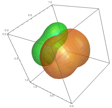
ContourPlot3D[{p1[x, y, z] == density1, p2[x, y, z] == density2}, {x, 
  0, 1}, {y, 0, 1}, {z, 0, 1.1}, Mesh -> None, 
 ContourStyle -> {Directive[Orange, Opacity[0.5], 
    Specularity[White, 30]], 
   Directive[Green, Opacity[0.5], Specularity[White, 30]]}]

3D distribution CI

Cheers, Max

Posted 3 years ago

You were almost there. A way to determine the contour to encompass a specified proportion of the points is the following:

proportion = 0.95;
density = Sort[PDF[dist2, #] & /@ data1][[Floor[(1 - proportion)*Length[data1]]]];

This should work for the 3D case also. An alternative approach (if you really have independent random samples from some distribution) is to find the contour that encompasses some proportion of the area or volume). Both approaches are widely used when finding home ranges for animals.

Here is the complete code:

dist1 = MixtureDistribution[{1, 2, 1}, {BinormalDistribution[{0.2, 0.3}, {0.05, 0.1}, 0], 
    BinormalDistribution[{0.6, 0.7}, {0.1, 0.05}, 0], BinormalDistribution[{0.7, 0.5}, {0.03, 0.1}, 0]}];
data1 = RandomVariate[dist1, 1000];
dist2 = SmoothKernelDistribution[data1, {0.05, 0.05}];

proportion = 0.95;
density = Sort[PDF[dist2, #] & /@ data1][[Floor[(1 - proportion)*Length[data1]]]];

Show[ListPlot[data1, AspectRatio -> 1],
 ContourPlot[PDF[dist2, {x, y}], {x, 0, 1}, {y, 0, 1}, Contours -> {density}, 
 ContourShading -> None, PlotPoints -> 50]]

Data on contour encompassing 95% of the data

POSTED BY: Jim Baldwin

Hello Claude, thanks for the suggestion. But this gives only elliptic regions, as expected from a normal distribution. I tried a few things with SmoothKernelDistribution and ContourPlot and came up with a not very elegant and slow solution:

dist1 = MixtureDistribution[{1, 2, 
    1}, {BinormalDistribution[{0.2, 0.3}, {0.05, 0.1}, 0], 
    BinormalDistribution[{0.6, 0.7}, {0.1, 0.05}, 0], 
    BinormalDistribution[{0.7, 0.5}, {0.03, 0.1}, 0]}];
data1 = RandomVariate[dist1, 1000];
ListPlot[data1, PlotRange -> {{0, 1}, {0, 1}}, AspectRatio -> 1]
SmoothDensityHistogram[data1, {0.05, 0.05}, 
 PlotRange -> {{0, 1}, {0, 1}}]
dist2 = SmoothKernelDistribution[data1, {0.05, 0.05}];
p[x_, y_] = PDF[dist2, {x, y}];
c1 = ContourPlot[p[x, y], {x, 0, 1}, {y, 0, 1}, Contours -> {0.46}, 
  ContourShading -> None, PlotPoints -> 50]
g1 = FullGraphics[c1];
regs = Polygon[g1[[1, 1, 1, 1, #]]] & /@ 
   Drop[g1[[1, 1, 1, 2, 2, 2, 1]], 1][[All, 1]];
Show[Graphics[regs], PlotRange -> {{0, 1}, {0, 1}}, AspectRatio -> 1]
Plus @@ (NIntegrate[p[x, y], {x, y} \[Element] #, 
     WorkingPrecision -> 10] & /@ regs)

The problem is that setting the level for the contour to get the 95% level (here set at 0.46) is trial and error. Maybe someone has a better and faster code.

Thanks for your input!

Max

Hello! Try something like:

Needs["MultivariateStatistics`"];

data = RandomReal[MultinormalDistribution[{1, 15}, v], {1000}];
\[CapitalOmega] = EllipsoidQuantile[data, 0.95];
Show[ListPlot[data, Frame -> True, AspectRatio -> Automatic], 
 Graphics[\[CapitalOmega]]]
POSTED BY: Claude Mante
Reply to this discussion
Community posts can be styled and formatted using the Markdown syntax.
Reply Preview
Attachments
Remove
or Discard

Group Abstract Group Abstract