Hi,
I will be more specific, starting the problem since begining:
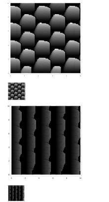
1)I have these images (map of force due a potential, Fx and Fy) that I need to replicate the last two , using mathematica ( my adviser wanted to use Fortran..., but I am fighting to consolidate Mathematica coding in my department )

The potential that I need to Minimize at each step is:
-V *(2 Cos[(2 Pi x)/a]*
Cos[(2 Pi y)/(a Sqrt[3])] + Cos[(4 Pi y)/(a Sqrt[3])]) + (k/2)*(X- x)^2 + (k/2)*(Y - y)^2
So, when I get the minima, or (x,y) positions, they will be used to the next step. I use them like that:
first step:
i(=X) = 0 and j (=Y)=0, -> potential minimized -> x,y calculated.
second step:
i= 0 j=1, potential minimized using the last (x,y).....-> "new" x,y calculated..
and so on...
And I am going collecting at each step the pairs (x,y) , that will be used to calculate the Map Forces Fx and Fy.
At the final I have an output.txt with all x,y, collected. and I use x for calculate Fx and y for calculate Fy.
and finally I make a table to plot Fx x X(or i) and Fy x Y(or j)
obs: "F = k* x" (oscilator)
well, and I did a lot of tests (since august....) and the best images I could get (using contourplot) were (for Fx, and Fy, respectively)
The parameters:
(*a= 2.46 \[Angstrom] = 2.46 10^-10m*)
(*k= 25 N/m as 1 joule = N.m, so , N/m= eV/(16 \[Angstrom]^2)*)
And the code is that:
$HistoryLength = 0;
ClearSystemCache[];
ClearAll["Global`*"];
SetDirectory["/home/marcelo/Documentos/Tomlinson/"];
Block[{x, y, i, j, FmolaX, FmolaY, c = {0, 0}, a = 2.46, k = 1.5625,
V = 0.5},
Emin[go_, ho_] :=
Module[{g = go, h = ho}, {x, y} /.
Take[Flatten[
N[FindMinimum[-V *(2 Cos[(2 Pi x)/a]*
Cos[(2 Pi y)/(a Sqrt[3])] +
Cos[(4 Pi y)/(a Sqrt[3])]) + (k/2)*(x - g)^2 + (k/
2)*(y - h)^2, {{x, First[c]}, {y, Last[c]}},
Method -> "PrincipalAxis"], 7]], -2]];
Do[
If[j == 0, c = {0, i}]; (*<- to avoid contour problems in the beginning of the step, I can´t use the last x,y results, for the next i*)
c = Emin[j, i] ;
FmolaX = -16*k*(First[c] - (j))*(10^-10);
FmolaY = -16*k*(Last[c] - (i))*(10^-10);
{FmolaX, FmolaY} >>> "DataFxFyTomlinsonV20.txt";
c >>> "DataMinimTomlinsonV20.txt",
(*Print[
"the minima of the function related to step Y",i," X",j,":",
c],*) {i, 0.0, 10.0, 0.1}, {j, 0.0, 10.0, 0.1}]
];
If you can see, I did steps of 0.1, and each step I used the last pair of {x,y},of the minimized potential.
As my images were not so good, mainly Fy, I tried aplying the gradient :
F=-\[Del](x,y) Subscript[E, tot]
So , I got two eqautions from the potential, and then I tested NSolve for Fx=0 and Fy = 0.
Details, When I tested the model 1d worked fine! See below:
equauni =
Quiet[NSolve[(2 \[Pi] )/ a Subscript[V, z] Sin[(2 \[Pi] x)/a] +
k (x - #) == 0, x, Reals] & /@
Table[i, {i, 0, 10, 0.02}] /. {a -> 246/100, k -> 25/16,
Subscript[V, z] -> 5/10}] >> datateste1
equauni2 = Flatten[Take[{x} /. equauni // Simplify, All, 1]];
dataequani = Transpose[{Table[i, {i, 0, 10, 0.02}], equauni2}];
Map[Length, {equauni2}];
Map[Length, {Table[i, {i, 0, 10, 0.02}]}];
ListPlot[Tooltip[Transpose[{Table[i, {i, 0, 10, 0.02}], equauni2}]],
PlotStyle -> Green,
AxesLabel -> {Subscript[x, 0][\[Angstrom]], x[\[Angstrom]]}]
And calculating the Force:
Fmola[x_,
d_] := -k (x -
d)*(10^-10);(*converted to Newton (N)*)
ListPlot[Tooltip[
Transpose[{ 10^-10 equauni2,
Fmola[equauni2, Table[i, {i, 0, 10, 0.02}]] /. {a -> 246/100,
k -> 25/1, Subscript[V, z] -> 5/10}}]],
AxesLabel -> {x["m"], F["N"]}, AxesOrigin -> {0, 0},
PlotRange -> All, ImageSize -> Large, PlotStyle -> Green, Mesh -> All]
I hope, this explanation can be more useful.


