Message Boards Message Boards

Error in NDSolveValue[ ]: solve the heat equation in 2D?

Posted 3 years ago

Dear All, As I'm learning Mathematica, I encountered troubles I can't seem to solve on my own. Here's My code :

Clear["Global`*"];
HeatEq = \!\(
\*SubscriptBox[\(\[PartialD]\), \(t\)]\(T[x, y, t]\)\) == Laplacian[
   T[x, y, t],{x, y}];
L = 2; l = 1/2; tmax = 15;
\[CapitalOmega] = Rectangle[{0, 0}, {L, l}];
boundaries = {T[x, y, 0] == 5, T[0, y, t] == 0, T[L, y, t] == 0, 
   T[x, 0, t] == 0, T[x, l, t] == 0};
boundaries2 = {DirichletCondition[T[x, y, t] == 0, True], 
   T[x, y, 0] == 5};
sol = NDSolveValue[Join[{HeatEq}, boundaries2], 
   T, {x, y} \[Element] \[CapitalOmega], {t, 0, tmax}];
Animate[DensityPlot[
  sol[x, y, t], {x, y} \[Element] \[CapitalOmega]], {t, 0, tmax}]

As you wander through my code, here is what it is supposed to do :

  • Clear all variables previously used, and define the Heat equation in 2 dimensions of space
  • Define the rectangle I'm going to cool down.
  • Define the boundaries (0°C on the edges, 5°C elsewhere)
  • Solve the equation, and get the temperature.
  • Plot an animation over time of the cooling

If facing two major issues here. The first one concerns the boundaries conditions. When I use the DirichletCondition, it seems to work "on its own", and yet produces strange results (Where the boundaries are not respected in the simulation). Moreover, As you can see I defined an original boundary condition, and exposing all of them, edge per edge. Yet this one doesn't work, and I really don't understand why. It produces the message : "Boundary condition T[x,1/2,t]==0 is not specified on a single edge of the boundary of the computational domain".

In a second time, I just can't seem to find how you fix a color scale for the integrity of a sequence of density plot. I want to have each color affected to a single value of temperature, for every density plot in a list. And after hours of testing of changes for ColourFunction, I got nothing viable.

I've been searching on the web for hours, and I can't find any solution. Would you kindly help me? I'm looking forward to your answers!

Kind Regards.

6 Replies

Dear Neil,

Thank you for the clarification of point 2 (now it makes sense!) and for the nice tip of point 1.

Regards,

Lissa.

For a first introduction to the Wolfram community, I have to say that I am truly impressed by your dedication. Thanks a lot Lissa and Neal. I took notes from your proposition, and I ended up with a fairly great simulation. Moreover, the links for the Methods of Line and Finite Element Method will keep me busy for at least two weeks, but I am sure they will pay off.

With my gratitude,

Alexandre

Alexandre,

Lissa gave an excellent answer. Just a few minor points to add that might help.

  1. you can get the right shape for your animation adding AspectRatio->Automatic to the DensityPlot. It will look like a rectangle instead of a square.

  2. Addressing Lissa's comments about the difference between boundaries and boundaries2: By using boundaries, Mathematica solves the PDE using Method of Lines. By using boundaries2, Mathematica uses the Finite Element Method. This is why you can't integrate over a region using boundaries (vs boundaries2) This distinction is important because you might want to specify additional options for each of the methods. Method of Lines can be found here, Finite Element Method can be found here.

I hope this helps.

Regards,

Neil

POSTED BY: Neil Singer

The strangeness is just a manifestation of the number of points considered to make the plot. To get rid of the triangles you can just set the option PlotPoints of the DensityPlot to some number higher than the default; I think PlotPoints->50 might be enough for you. Also, I exported the animated output to a gif, by:

p = Animate[DensityPlot[sol[x, y, t], {x, y} \[Element] \[CapitalOmega], PlotLegends ->BarLegend[{Automatic, {0, 5}}, 50], ColorFunctionScaling -> False, PlotPoints -> 50], {t, 0, 1/10}];

Export["nodrop.gif",p];

and then there is no framerate drop. Though it did take my computer 94 seconds for that. I don't know how to enhance its performance, but maybe this helps.

A huge thank you Lissa, It is exactly what I intended to do ! I'd still wonder why the border evolution appears so strange with all those triangles. Any Idea of how I can improve that ?

I also encounter framerates drop, it doesn't appear smoothly, have you got a recommandation to enhance performance of the plot ?

Once again, thank you very much for your time !

First, the initial condition is also being applied at the boundary---hence the error message. To fix that, instead of T[x,y,0]== 5, you can write:

T[x,y,0]==If[x==0||x==L||y==0||y==l,0,5]

With that, your code using ''boundaries2'' works fine.

Now, to use ''boundaries'' , beyond fixing implementation of the initial condition, if you replace, in the argument of NDSolveValue,

{x, y} \[Element] \[CapitalOmega]  

by

{x, 0, L}, {y,0, l} 

then it works fine as well. I don't know why, though. I had never defined the domain of an equation using a region like you did, it's interesting..

So, it reads:

HeatEq = \!\(
\*SubscriptBox[\(\[PartialD]\), \(t\)]\(T[x, y, t]\)\) == Laplacian[
       T[x, y, t], {x, y}];
L = 2; l = 1/2; tmax = 15;
\[CapitalOmega] = Rectangle[{0, 0}, {L, l}];
boundaries = {T[x, y, 0] == 
    If[x == 0 || x == 2 || y == 0 || y == 1/2, 0, 5], 
   T[0, y, t] == 0, T[L, y, t] == 0, 
      T[x, 0, t] == 0, T[x, l, t] == 0};
boundaries2 = {DirichletCondition[T[x, y, t] == 0, True], 
      T[x, y, 0] == If[x == 0 || x == 2 || y == 0 || y == 1/2, 0, 5]};
sol = NDSolveValue[Join[{HeatEq}, boundaries], 
      T, {x, 0, L}, {y, 0, l}, {t, 0, tmax}];
Animate[DensityPlot[
    sol[x, y, t], {x, y} \[Element] \[CapitalOmega]], {t, 0, tmax}, 
 AnimationRunning -> False]

Regarding the visualization. To check that things make sense, you can use:

ListAnimate@Table[Plot3D[sol[x, y, t], {x, 0, L}, {y, 0, l}], {t, 0, 2/10, 1/100}]

And if you set ``ColorFunctionScaling -> False'' in the DensityPlot, then it won't apply a different scaling for each DensityPlot. Since it cools down fast, I chose the range {t, 0, 1/10}) and, adding a fixed legend:

Animate[DensityPlot[sol[x, y, t], {x, y} \[Element] \[CapitalOmega], PlotLegends -> BarLegend[{Automatic, {0, 5}}, 50], ColorFunctionScaling -> False], {t, 0, 1/10}]

It looks like:
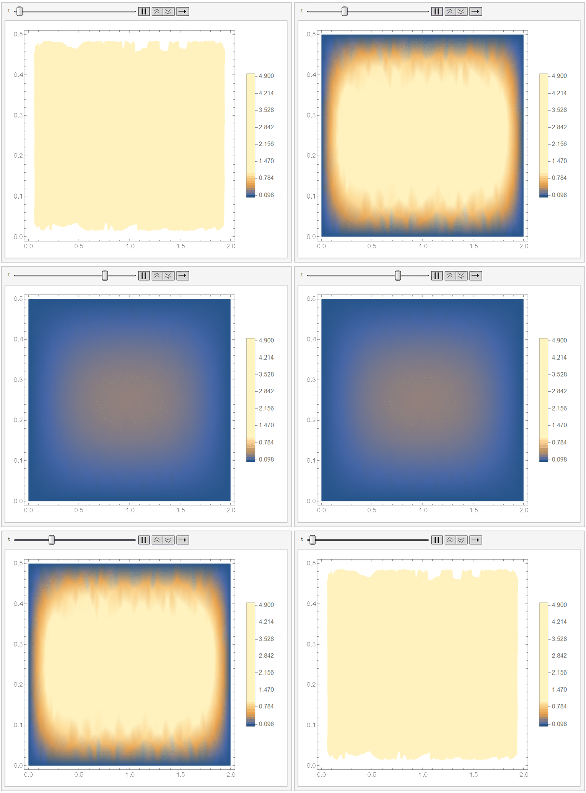
gif

Reply to this discussion
Community posts can be styled and formatted using the Markdown syntax.
Reply Preview
Attachments
Remove
or Discard

Group Abstract Group Abstract