This is a snippet from a strategy backtesting system that I am currently building in Mathematica.

One of the challenges when building systems in WL is to avoid looping wherever possible. This can usually be accomplished with some thought, and the efficiency gains can be significant. But it can be challenging to get one's head around the appropriate construct using functions like FoldList, etc, especially as there are often edge cases to be taken into consideration.

A case in point is the issue of calculating the profit and loss from individual trades in a trading strategy. The starting point is to come up with a FoldList compatible function that does the necessary calculations:

CalculateRealizedTradePL[{totalQty_, totalValue_, avgPrice_, PL_, 
totalPL_}, {qprice_, qty_}] := 
Module[{newTotalPL = totalPL, price = QuantityMagnitude[qprice], 
newTotalQty, tradeValue, newavgPrice, newTotalValue, newPL}, 
newTotalQty = totalQty + qty;
tradeValue = 
If[Sign[qty] == Sign[totalQty] || avgPrice == 0, price*qty, 
If[Sign[totalQty + qty] == Sign[totalQty], avgPrice*qty, 
price*(totalQty + qty)]];
newTotalValue = 
If[Sign[totalQty] == Sign[newTotalQty], totalValue + tradeValue, 
newTotalQty*price];
newavgPrice = 
If[Sign[totalQty + qty] == 
Sign[totalQty], (totalQty*avgPrice + tradeValue)/newTotalQty, 
price];
newPL = 
If[(Sign[qty] == Sign[totalQty] ), 0, 
totalQty*(price - avgPrice)];
newTotalPL = newTotalPL + newPL;
{newTotalQty, newTotalValue, newavgPrice, newPL, newTotalPL}]

Trade P&L is calculated on an average cost basis (as opposed to FIFO or LIFO).

Note that the functions handle both regular long-only trading strategies and short-sale strategies, in which (in the case of equities), we have to borrow the underlying stock to sell it short. Also, the pointValue argument enables us to apply the functions to trades in instruments such as futures for which, unlike stocks, the value of a 1 point move is typically larger than $1 (e.g. $50 for the ES S&P 500 mini futures contract).

We then apply the function in two flavors, to accommodate both standard numerical arrays and timeseries (associations would be another good alternative):

CalculateRealizedPLFromTrades[tradeList_?ArrayQ, pointValue_ : 1] := 
Module[{tradePL = 
Rest@FoldList[CalculateRealizedTradePL, {0, 0, 0, 0, 0}, 
tradeList]}, 
tradePL[[All, 4 ;; 5]] = tradePL[[All, 4 ;; 5]]*pointValue;
tradePL]
CalculateRealizedPLFromTrades[tsTradeList_, pointValue_ : 1] := 
Module[{tsTradePL = 
Rest@FoldList[CalculateRealizedTradePL, {0, 0, 0, 0, 0}, 
QuantityMagnitude@tsTradeList["Values"]]}, 
tsTradePL[[All, 4 ;; 5]] = tsTradePL[[All, 4 ;; 5]]*pointValue;
tsTradePL[[All, 2 ;;]] = 
Quantity[tsTradePL[[All, 2 ;;]], "US Dollars"];
tsTradePL = 
TimeSeries[
Transpose@
Join[Transpose@tsTradeList["Values"], Transpose@tsTradePL], 
tsTradeList["DateList"]]]

These functions run around 10x faster that the equivalent functions that use Do loops (without parallelization or compilation, admittedly)

Let's see how they work with an example:

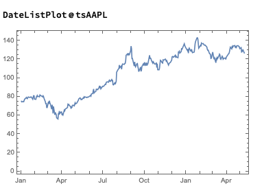
tsAAPL = FinancialData["AAPL", "Close", {2020, 1, 2}]    

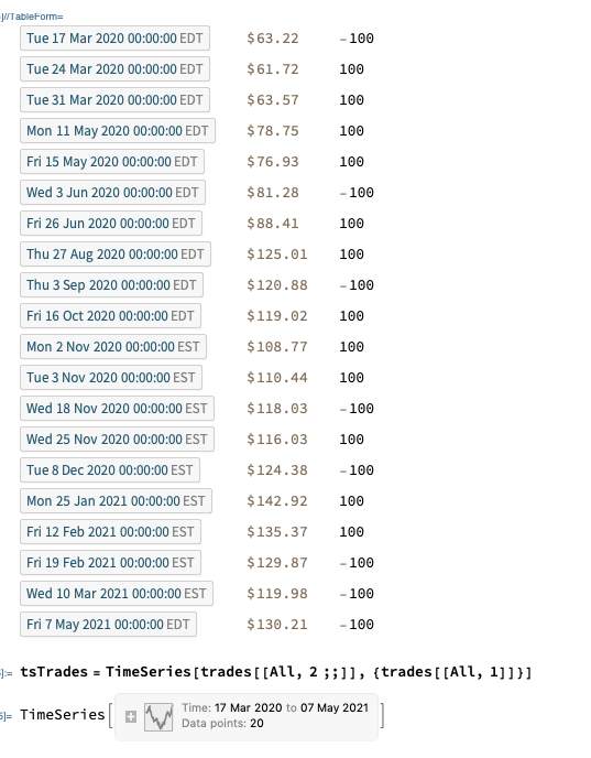
Next, we'll generate a series of random trades using the AAPL time series, as follows (we also take the opportunity to convert the list of trades into a time series, tsTrades):

trades = Transpose@
   Join[Transpose[
     tsAAPL["DatePath"][[Sort@
        RandomSample[Range[tsAAPL["PathLength"]], 
         20]]]], {RandomChoice[{-100, 100}, 20]}];
trades // TableForm

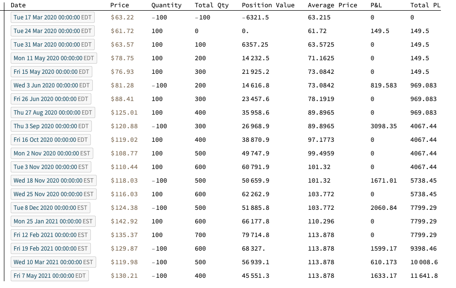
We are now ready to apply our Trade P&L calculation function, first to the list of trades in array form:

TableForm[
Flatten[#] & /@ 
Partition[
Riffle[trades, 
CalculateRealizedPLFromTrades[trades[[All, 2 ;; 3]]]], 2], 
TableHeadings -> {{}, {"Date", "Price", "Quantity", "Total Qty", 
"Position Value", "Average Price", "P&L", "Total PL"}}]

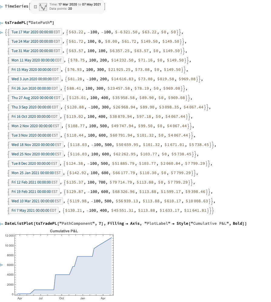
The timeseries version of the function provides the output as a timeseries object in Quantity["US Dollars"] format and, of course, can be plotted immediately with DateListPlot (it is also convenient for other reasons, as the complete backtest system is built around timeseries objects):

tsTradePL = CalculateRealizedPLFromTrades[tsTrades]

So far so good - but this only covers calculation of the realized profit and loss. I will leave the calculation of unrealized gains and losses for another post.