Over on Stack Exchange a user posted the following question:

This is a basic question about using the KalmanFilter function. I want to use the KalmanFilter function (or other related Kalman Filter functions in Mathematica) to estimate the time-varying beta(t) in the linear model:

AAPL (t) = beta (t) * SP500 (t) + e (t)

Where e(t) is a random error process.

I have tried the following:

AAPL = FinancialData["AAPL", "Return", {2020, 1, 2}];
SP500 = FinancialData["GSPC", "Return", {2020, 1, 2}];
tds = TemporalData[{AAPL, SP500}];
tsm = TimeSeriesModelFit[tds] // Quiet;
Kf = KalmanFilter[tsm];
DateListPlot[Kf]

which produces the following:

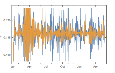
But it's not the result I am looking for.

I am unclear as to how to formulate the problem in a way that will produce estimates of beta(t) using Mathematica's KalmanFilter function (or other Kalman-related functions).

My answer shows one way to handle the problem (see below), but its doesn't address the question directly of how to apply the Wolfram Language KalmanFilter function (or other Kalman-related functions) to produce the same result more efficiently than my code.

Does anyone in the community have an idea how it can be done?

KalmanTimeLoop[Y_, X_, a_, b1_, Ve_, Vw_, Covb1_] := 
 Module[{Yhat, b, k, n, e, t, Q, K, Covb, Zscore},
  (************************************************************) 
  (************************************************************) 
  (** UPDATES THE KALMAN FILTER PARAMETERS FOR EACH TIMESTEP ***)
  (************************************************************) \

  (*                                                        
  X = k x n matrix of k prices data series for t = 1,...,n ;
      note that X(t)[[1,All]] = 1 for all t;
  a = k x k State Transition matrix estimated in initialization;
  b = k x n matrix of state vectors b(t) = {b1,...,bk},
  Ve = scalar price error variance, estimated in initialization;
  Vw = k x k state noise covariance matrix, 
  estimated in initialization;
  Covb[[t]] = k x k state covariance matrix at time t = 1,...,n;
  *)
  (***********************************************************) 

  {k, n} = Dimensions@X;
  e = ConstantArray[0, n];
  Q = ConstantArray[0, n];
  b = ConstantArray[0, {k, n}];
  Covb = ConstantArray[0, {n, k, k}];
  b[[All, 1]] = b1;
  Covb[[1]] = Covb1;
  Do[
   (*************************************************)
   (* 
   update state prediction and state covariance matrix*)

   If[t > 1, b[[All, t]] = a . b[[All, t - 1]];
    Covb[[t]] = a . Covb[[t - 1]] . Transpose[a] + Vw;
    Covb[[t]] = DiagonalMatrix@Diagonal@Covb[[t]];];
   (*************************************************)
   (* 
   Measurement Prediction Equation *)

   Yhat = X[[All, t]] . b[[All, t]];
   (*************************************************)
   (* 
   Measurement Prediction Error *)
   e[[t]] = Y[[t]] - Yhat;
   (*************************************************)
   (* 
   Measurement Covariance Prediction *)     
   Q[[t]] = X[[All, t]] . Covb[[t]] . X[[All, t]] + Ve; 
   (*************************************************)
    (* 
   Kalman Gain *)                  
   K = Covb[[t]] . X[[All, t]]/Q[[t]];  
   (*************************************************) 
   (* State Update *)
   b[[All, t]] = b[[All, t]] + K*e[[t]];
   (*************************************************) 
   (* State Covariance Update *)                  
   Covb[[t]] = 
    Covb[[t]] - DiagonalMatrix[K*X[[All, t]]] . Covb[[t]]; 
   (*************************************************) 
   , {t, 1, n}];
  Zscore = e/Sqrt[Q];
  {b, Covb, K, e, Q, Zscore}]