Message Boards Message Boards

Inaccuracy of the solution from Lorentzian dielectric function

Posted 3 years ago

Hi Wolfram community!

So here's my situation. I wrote a simple code that plots the dielectric function / optical constants using a multi-oscillator Lorentz equation. To verify my code, I tried running it using known parameters that have also shown the resulting dielectric function / optical constants. However, the plots I'm getting from the code is a bit different from the correct plots. The shape of the curves are the same. However, values are not 100% correct. it is a little bit off. Also, for the imaginary part, the plot is negative even when the correct answer must be positive. I just want to ask what could be the possible reason why the solution I'm getting from my code is like this?

Here's my code:

n = 2.481; (*Einf*)
c1 = 0.00623; (*amplitude*)
a1 = 1.687; (*resonant energy (eV)*)
b1 = 0.122; (*damping coefficient*)

c2 = 0.0170;
a2 = 1.868;
b2 = 0.127;

c3 = 0.00825;
a3 = 2.648;
b3 = 0.0717;

c4 = 0.0109;
a4 = 2.789;
b4 = 0.162;
model1[x_] := 
 Sqrt[ n + ((c1)/((a1*a1) - (x*x) + (I*b1*x))) + ((c2)/((a2*a2) - (x*
         x) + (I*b2*x))) + ((c3)/((a3*a3) - (x*x) + (I*b3*
         x))) + ((c4)/((a4*a4) - (x*x) + (I*b4*x)))]

Plot[Re[model1[x]], {x, 0.60, 6.50}, PlotLabel -> "n vs. energy"]
Plot[Im[model1[x]], {x, 0.60, 6.50}, PlotLabel -> "k vs. energy"]

Thank you in advance for helping me!

Edit: I've also put the resulting plots and the reference plot here: Plots from Mathematica code: enter image description here

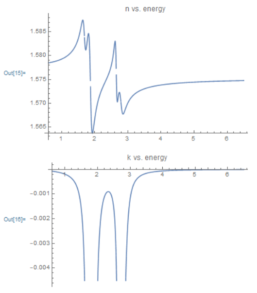
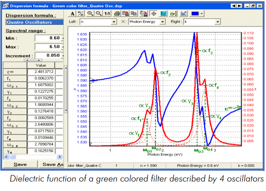
Reference plot (From Horiba's Lorentz Dispersion Model) enter image description here

POSTED BY: Phoebe Perez
4 Replies
Posted 3 years ago

Thank you very much, Dr. Lichtblau!

POSTED BY: Phoebe Perez

There is neither plot nor a set of reference values to contrast with. Please provide some values that are off, along with the expected values and some reason for why they are correct.

POSTED BY: Daniel Lichtblau
Posted 3 years ago

Hi, Dr. Lichtblau.

I have edited my post to include the images of the plots and the reference. Thanks!

POSTED BY: Phoebe Perez

One issue is the formula. There are squares missing in the numerator. Check the section "Extension to multiple oscillators" here. Plots will look better if you change the model as below.

model1[x_] := 
 Sqrt[n + ((c1*a1^2)/((a1*a1) - (x*x) + I*b1*x)) + ((c2*
       a2^2)/((a2*a2) - (x*x) + (I*b2*x))) + ((c3*
       a3^2)/((a3*a3) - (x*x) + (I*b3*x))) + ((c4*
       a4^2)/((a4*a4) - (x*x) + (I*b4*x)))]

I do not know how to account for the sign of the imaginary part. But you can get the expected plots like so:

ResourceFunction["MultipleAxesPlot"][
 Evaluate[{1, -1}*ReIm[model1[x]], {x, 0.60, 3.50}, 
  PlotLabel -> "n and k vs. energy", PlotRange -> All, 
  PlotPoints -> 150]]

enter image description here

POSTED BY: Daniel Lichtblau
Reply to this discussion
Community posts can be styled and formatted using the Markdown syntax.
Reply Preview
Attachments
Remove
or Discard

Group Abstract Group Abstract