Message Boards Message Boards

14
|
20647 Views
|
2 Replies
|
18 Total Likes
View groups...
Share
Share this post:

1D quasicrystals by Fibonacci substitution and lattice projection

Posted 10 years ago
Quasicrystals  ( Nobel Prize in Chemistry in 2011 ) are structures that are build from finite set of primitive units, perfectly ordered but aperiodic. Let's consider one dimensional (1D) case of the following substitution system: 

S -> L
L -> LS

Or, a shorter stick transforms to longer one, and a longer stick is replaced by a pair of long and short ones. Mathematica code is easy to write, here are two basic versions with symbols and strings giving same result:

Grid[NestList[Flatten[# /. {S -> L, L -> {L, S}}] &, {S}, 9], Spacings -> {0, 0}]


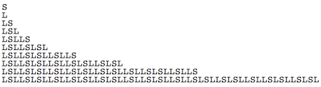
Column[NestList[StringReplace[#, {"o" -> "-", "-" -> "-o"}] &, "-", 8], Spacings -> 0]


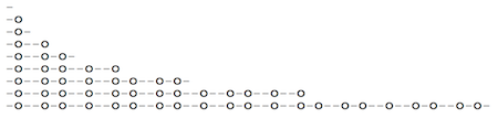
We can continue this substitution process infinitely and in this limit ratio of fraction of longer to shorter pieces goes to Golden Ratio. Not surprising, - number of L's and S's in sequential generations is given by Fibonacci numbers. And the problem is identical to Fibonacci Rabbits setup.

Interesting part is that sequence of L's and S's is perfectly ordered (predictable) but is aperiodic. Meaning one cannot find a finite sub-sequence to shift it repeatedly in order to recover the whole L-S-... chain. In other words - there is no translational symmetry. This is called Quasicrystal. Now even more surprising fact is that the same sequence can be obtained by projecting regular lattice dimension D on a manifold dimension D-k. For example projecting 2D grid on a line. If a line is at an irrational slope that avoids any lattice plane, then nearest lattice points projected on the line will slice it into quasicrystal sequence.


 Animate[
  Module[{grid, f, lndat, near, lnpts, lines, bnd1, bnd2},
  
   grid = Flatten[Outer[List, Range[-6, 6], Range[-6, 6]], 1];
   f[x_] := m x;
   lndat =
    Select[{#, f[#]} & /@ Range[-6, 6, .01], -6 < #[[2]] < 6 &];
   near = Union[Flatten[Nearest[grid, #] & /@ lndat, 1]];
   lnpts = First[Nearest[lndat, #]] & /@ near;
  lines = Line /@ Thread[{near, lnpts}];
 
  Show[Plot[f[x], {x, -4, 4}, PlotRange -> 4],
   Graphics[{{Opacity[.7], PointSize[.017], Point[grid]}, {Red,
      Opacity[.5], PointSize[.03], Point[near]}, {Orange,
      Thickness[.005], lines}, {PointSize[.015], Blue,
      Point[lnpts]}}], AspectRatio -> 1]],

{{m, -4, "slope"}, -4, 4}, AnimationRunning -> False,
AnimationRate -> .5]

Or adding band of nearest points ( see code at the end ):


What happens when we go from 1D to 2D quasicrystals? Well thing get a bit more complicated. A bit history from Wikipedia:
In 1961, Hao Wang asked whether determining if a set of tiles admits a tiling of the plane is an algorithmically unsolvable problem or not. He conjectured that it is solvable, relying on the hypothesis that any set of tiles, which can tile the plane can do it periodically (hence, it would suffice to try to tile bigger and bigger patterns until obtaining one that tiles periodically). Nevertheless, two years later, his student, Robert Berger, constructed a set of some 20,000 square tiles (now called Wang tiles), which can tile the plane but not in a periodic fashion. As the number of known aperiodic sets of tiles grew, each set seemed to contain even fewer tiles than the previous one. In particular, in 1976, 
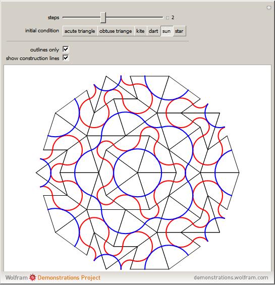
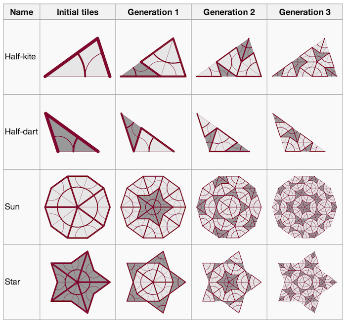
Roger Penrose proposed a set of just two tiles, up to rotation, (referred to as Penrose tiles) that produced only non-periodic tilings of the plane. These tilings displayed instances of fivefold symmetry.

Can Penrose Tiling be obtained by projection? Yes! In 1981, De Bruijn explained a method in which Penrose tilings are obtained as 2D projections from a 5D cubic structure. Explore tilings at the Wolfram Demonstrations, in particular, take a look at beautiful "Penrose Tiles" from Stephen Wolfram, Lyman Hurd, and Joe Bolte:


Appendix: code for 1D quasicrystal with bands

 Animate[
  Module[
   {grid, f, lndat, near, lnpts, lines, bnd1, bnd2},
 
   grid = Flatten[Outer[List, Range[-6, 6], Range[-6, 6]], 1];
 
   f[x_] := m x;
 
   lndat =
   Select[{#, f[#]} & /@ Range[-6, 6, .01], -6 < #[[2]] < 6 &];

  near = Union[Flatten[Nearest[grid, #] & /@ lndat, 1]];

  lnpts = First[Nearest[lndat, #]] & /@ near;

  lines = Line /@ Thread[{near, lnpts}];

  {bnd1[x], bnd2[x]} =
   m x + (#2 -
        m #1) & @@@ (Sort[#,
         EuclideanDistance @@ #1 > EuclideanDistance @@ #2 &] & /@
       GatherBy[
        Thread[{near, lnpts}], #[[1, 1]] - #[[2, 1]] > 0 &])[[All, 1,
      1]];

  Show[
   Plot[Evaluate@{f[x], bnd1[x], bnd2[x]}, {x, -4, 4}, PlotRange -> 4,
     PlotStyle -> {Automatic, Dashed, Dashed},
    Filling -> {2 -> {3}}],
   Graphics[{
     {Opacity[.5], PointSize[.015], Point[grid]},
     {Red, Opacity[.5], PointSize[.03], Point[near]},
     {Orange, Thickness[.005], lines},
     {PointSize[.015], Blue, Point[lnpts]}}]
   , AspectRatio -> 1]
  ]
, {{m, -4, "slope"}, -4, 4}, AnimationRunning -> False,
AnimationRate -> .5]
POSTED BY: Vitaliy Kaurov
2 Replies
Hi Vitaliy,

Your post has some pretty good information, especially for beginners, but I think a few points could use improvement or refinement. It would be nice to spell out a connection between the typographical patterns and pictorial patterns. Those connections are presented nicely by Grimm and Schreiber, in a 1999 article with Mathematica code ( http://arxiv.org/pdf/cond-mat/9903010v1.pdf ). Figure 4.2 of this paper shows the staircase in a window of fixed width. In their depiction you can see plainly that the horizontal and vertical segments of the staircase are related to the long and short sequences generated by the typographical rules. With fixed window, it is also possible to introduce noise into the sequence, as is done neatly in Figure 4.3.

If you keep looking into aperiodic order, you will find that some people have gone beyond interest in just the few examples that have already found natural realizations. In another good article, some authors have asked: "Which distributions of matter diffract?" ( http://arxiv.org/pdf/math-ph/0301019v1.pdf ). I am hesitant to show any work that I am developing for publication, but I think I will share one function that I have computed, because I think it is a really great example of the expressive capability of Mathematica.

I never meant to make a dragon curve, but somehow I wrecked myself into doing just that. I should probably have been studying dielectrics. The function SetDragon makes a list of replacement rules that map the integers into a binary dragon sequence. This function requires the input of a root shift integer between 0 and 3, and a branching list of arbitrary length with elements either 0 or 1. It should make a function for every possible dragon sequence in the inverse limit where the length of the branching list approaches infinity and the sequence is completed.

 SetDragon[Root_, BinaryBranching_] := Append[Flatten[Reap[FoldList[
       (Sow[{x_Integer /;
             IntegerQ[
              Divide[(x - #1 - (2^#2[[2]]) BitXor[0, #2[[1]]]),
               2^(#2[[2]] + 1)]] :> 1,
           x_Integer /;
             IntegerQ[
              Divide[(x - #1 - (2^#2[[2]]) BitXor[1, #2[[1]]]),
               2^(#2[[2]] + 1)]] :> 0}
         ]; #1 + (2^#2[[2]]) BitXor[0, #2[[1]]] + 2^(#2[[2]] - 1)) &,
      Root, Transpose[{#, Range[Length@#]} &@BinaryBranching]]][[2]]
   ], _Integer :> "?"]

You can use this function to compare different dragon sequences as they appear, flying over all of the integers.

 BranchCompare = Column[{ArrayPlot[
      Map[
       Range[0, 20] /. SetDragon[0, #] &,
       {{0}, {0, 0}, {0, 0, 0}}
       ], Mesh -> True, ImageSize -> 500
      ],
     ArrayPlot[
      Map[
       Range[0, 20] /. SetDragon[0, #] &,
      {{0}, {0, 1}, {0, 1, 0}}
      ], Mesh -> True, ImageSize -> 500
     ]
    }];


I was somewhat surprised by a comparison of the sequences as actual dragon images. You can also use the function to look at completed sequences (words between nearest "?" symbols). For a branching list of length n, two sequences appear in the plane either as entirely overlapped dragons or as half-overlapped dragons, depending on the last element of the branching list.

 Graphics[
  MapThread[{#2,
     Line[{Re[#], Im[#]} & /@
       FoldList[Plus, 0,
        FoldList[Times, 1, Identity[#1] /. {1 -> -I, 0 -> I}]]]
     } &,
   {{
     Replace[
      Range[-4*2^10, 0] /. SetDragon[0, RandomInteger[{0, 1}, 11]],
     {__, "?", x__, "?", __} :> {x}],
    Replace[
     Range[0, 4*2^10] /. SetDragon[0, RandomInteger[{0, 1}, 11]],
     {__, "?", x__, "?", __} :> {x}]
    },
   {Darker@Red, Darker@Purple}
   }]
]


This result is reminiscent of the original work of Harter. Before he went out to visit Martin Gardner in New York, apparently he had done some research for NASA into getting the dragons snout to snout, tail to snout, etc. Harter was telling me yesterday that if I got another dragon in there it could have C4 symmetry. Of course he's right, but that isn't really the point...

The dragon sequences (more exactly, sequences related to the dragon sequence) can specify distributions of matter that diffract, according to equation (9) of the article above. The folded periodic sub-sequences should each have nice bragg peaks. Sub-sequences of larger period occur less frequently in the total sequence. According to these properties the diffraction seems unsurprising.

This folded periodic structure that enables diffraction is the key to making the function SetDragon work. Surprisingly, I have found some functionality that does not seem to be built in to Mathematica. Maybe someone will show me a better way to determine membership to subsets of the integers, but the hack of IntegerQ seems to work pretty well. Number systems are good to emphasize as they recur throughout the examples of hierarchical aperiodic order; though, some examples, including the icosahedral tilings, do not work out so easily. Even with regard to useful and normal topics, number systems should be emphasized, especially as they occur everywhere in practical fields such as measurement, analysis, etc.

If you find some interest in this calculation, you will probably be excited to read the paper I am working on, whenever it is finished and hopefully published. It's even more fun, and it should be accompanied by new, exploratory computations with more substance and detail.

Brad
POSTED BY: Brad Klee
Vitaliy,
This is a  beautiful example. I'd been wondering how to explain this concept efficiently to students--this is it. Thanks so much for sharing this.
WCC
POSTED BY: W. Craig Carter
Reply to this discussion
Community posts can be styled and formatted using the Markdown syntax.
Reply Preview
Attachments
Remove
or Discard

Group Abstract Group Abstract