You can extract x and y values and do a bit of Fourier analysis on those.

times = wsData["Times"];
values = QuantityMagnitude[wsData["Values"]];

Check whether, or to what extent, the measurement intervals are uniform.

gaps = Differences[times];
Tally[gaps]

(* {{86400, 3575}, {172800, 27}, {432000, 2}, {259200, 3}, {345600, 1}} *)

So there were some days when the apparatus was down or measurements were missed for other reasons. Also note that the main gap, 86400, is the seconds in one day.

Now check that the missing count is what we expect.

In[45]:= Length[times]

(* Out[45]= 3609 *)

In[44]:= missingtotal = 
 Total[Cases[
   Tally[gaps], {aa_ /; aa =!= 86400, bb_} :> bb*(aa/86400 - 1)]]

(* Out[44]= 44 *)

So that will account for the full 10 years, assuming three were leap years. A clean analysis would insert values into the gaps (using the mean, perhaps) and proceed from there. We will skip this step below and do a slightly cruder analysis.

Now find the period, which, not surprisingly, is one year. We extract the position of the largest frequency from Fourier (after making the mean zero), subtract 1 to account for position one being the DC component, and divide the adjusted length by that.

len = Length[values];
truelen = len + missingtotal
ft = Abs[Fourier[values - Mean[values]]];
max = Max[ft]
mainfreq = FirstPosition[ft, max][[1]] - 1
period = N[truelen/mainfreq]

(* 3653

48.3809

10

365.3 *)

We can (again, to crude approximation) clean this by removing small frequencies. By trial and error I arrived at the factor of 0.55 below. This retains two frequencies (plus their negative mirrors, at the other end of the list).

ftModified = Map[If[Abs[#] > .55*max, #, 0.] &, ft];
Position[ftModified, aa_ /; aa > 0]

(* {{8}, {11}, {3600}, {3603}} *)

Invert this clipped frequency list and create an interpolation.

inv = Re[InverseFourier[ftModified]];
interp = Interpolation[inv];

We can plot this.

Plot[interp[t], {t, 1, len}]

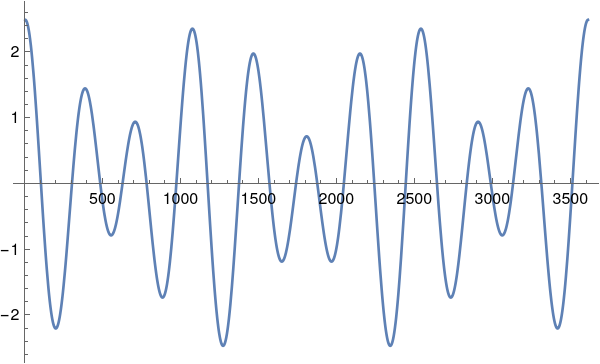
Using the secondary frequency indicates another possible period of around 522 days, by the way.