Vijay Arjun,
the main part of my approach was already done above by the approach of @Hans Dolhaine: This nice presentation of the dynamics implies that a fixed point (always?) has the form {x,x,x}, i.e. all coordinates have the same value. Assuming this to be true then the equations reduce to
$$
x'(t) = -b *x(t) +\sin(x(t))
$$
At a fixed point we have
$x'(t)=0$, which gives a simple relation between the fixed point coordinate
$x$ and the parameter
$b$:
$$
b=\frac{\sin(x)}{x}
$$
Next I calculate the eigenvalues of the respective Jakobian and put the above relation into:
ClearAll["Global`*"];
jackobian = {{-b, Cos[y], 0}, {0, -b, Cos[z]}, {Cos[x], 0, -b}};
(* eigenvalues of Jakobian: *)
ev = Refine[Re@Eigenvalues[jackobian /. {b -> Sinc[x], y -> x, z -> x}], x \[Element] Reals];
isneg = Boole[And @@ (Sign[#] < 0 & /@ ev)];
Plot[{ev, -isneg, Sinc[x]}, {x, 0, 23},
 PlotLabels -> {"ev1", "ev2", "ev3", None, "b"}, PlotStyle -> {Blue, Blue, Blue, Green, Red}, ImageSize -> 700, Filling -> {4 -> Axis}]
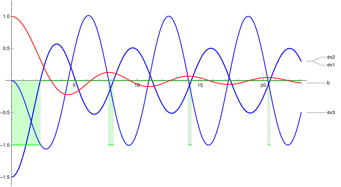
Here
$b$ and the real parts of the eigenvalues (depending on
$x$) are shown; the green bars are indicating the intervals where all these reals parts are negative - which is required for a fixed point to be stable/attractive.
And finally these intervals can be calculated:
(* Product of eigenvalues: *)
evProd = Times @@ ev;
(* reasonable starting points: *)
xstart = {2.1272, 7.73540, 8.04482, 14.1171, 14.3105, 20.34412, 20.49883};
(* intervals for possible fixed points: *)
xIntervals = BlockMap[Interval, Prepend[x /. FindRoot[evProd == 0, {x, #}] & /@ xstart, 0], 2];
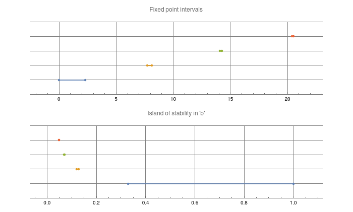
(* respective intervals for 'b' *)
bIntervals = Sinc[xIntervals];
GraphicsColumn[{NumberLinePlot[xIntervals, GridLines -> Automatic, PlotLabel -> "Fixed point intervals"],
NumberLinePlot[bIntervals, GridLines -> Automatic, PlotLabel -> "Island of stability in 'b'"]}, ImageSize -> 700]
I hope this is helpful - but in any case you should check my reasoning carefully!
Regards -- Henrik


