In order to study characteristics such as the monotonic value range of a function, it is necessary to draw the function and its guide function into the same coordinate system. for example: use this code can plot the function Plot[E^x (1 + x) + Cos[x], {x, -2, 2}] use such code can solve its guide function \!\( \SubscriptBox[\(\[PartialD]\), \(x\)]\(( \SuperscriptBox[\(E\), \(x\)]\ \((1 + x)\) + Cos[x])\)\) and plot it but how to when i input a function then the mathematica can solve its guide function ,and last draw the two function's images into the same coordinate. thx

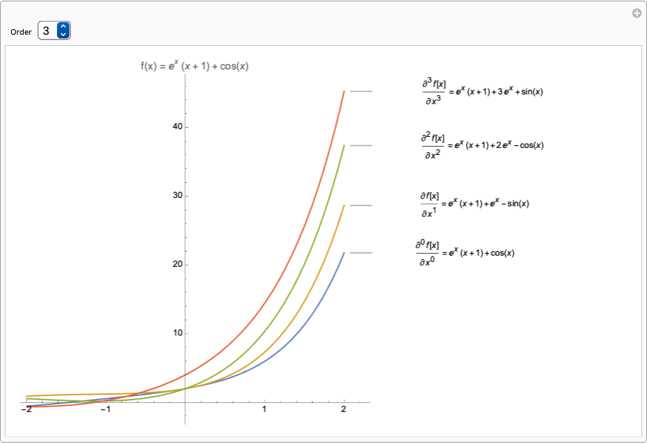
If you know how to differentiate then it is quite clear from the labels which order each curve corresponds to. Both can be displayed but the labels become long and high. The code is quite messy, good practice for you to refactor it to make it cleaner. Maybe you just want to display a number corresponding to the order rather than the differential operator, you can easily change the code to do that. Or maybe add a `Tooltip` to show the order, there are many possibilities.... Manipulate[ Refresh[ functions = Table[D[f[x], {x, n}], {n, 0, nMax, 1}]; orders = Table[D[f[x], {x, n}] // Inactivate // TraditionalForm // ToString, {n, 0, nMax, 1}]; labels = MapThread[#1 <> " = " <> ToString[#2, TraditionalForm] &, {orders, functions}];]; Plot[functions, {x, -2, 2}, PlotLabels -> labels, PlotRange -> All, ImageSize -> 700, AspectRatio -> 1, PlotLabel -> Row[{"f(x) = ", f[x]}]], {{nMax, 1, "Order"}, 1, 5, 1, PopupMenu}]

Thank you very much. That's what I want.

Specifically, it shows the function analytical expression of the derivative function in the image, and at the same time, it also shows the order of the derivative function of the original function. thx

Plot functions and their guide function images into same coordinate system