I've had an idea about looking at cellular automata in terms of directionalized correlation and computation inherent in the rulesets. I'll use Rule 30 as an example to help explain:
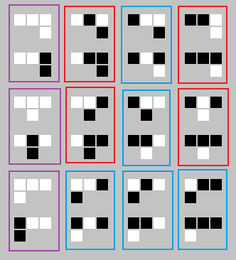
Explaining the above image: there are three major rows containing each of the 8 replacement rules, where the result has been aligned under a different column. Each rule has been paired with its matching counterpart, such that only the value of the replacement rule above the result cell differs. These pairs have rectangles drawn around them. The color of the rectangle indicates the type of relationship:
- Red rectangles mean information is lost relative to the cell above the result.
- Purple rectangles mean information is correlated with the cell above the result.
- Blue rectangles mean information is correlated and computation occurs (the value is changed).
At a glance, one can see the direction that information is correlated and computed. For Rule 30, information is highly-correlated and retained moving rightward, and has less correlation moving straight down or leftward.
This generalizes into cellular automata of more colors, range & dimensions, however I'm having a little difficulty comparing rules with higher amounts of colors, or putting a good scalar value on how much correlation and computation is taking place to determine if a particular cellular automaton is boring or not, though I have an idea on how to confirm a measurement is consistent.
A 1-range cellular automaton (like Rule 30) can be converted into a 2-range CA by taking it over two steps instead of one. The values for correlation and computation can be compared for consistency.
For example, the 2-range version of Rule 30 is rule 535945230, with each cell only 1/4 correlated with the two cells above-and-left, but 3/4 correlated with the two cells directly above and above-right, and 100% correlated with the cell above-and-far-right. This gives us the equations for correlation:
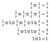
I'm using circle-operators as a stand-in for whatever multiplication-like and addition-like operations these should be. I'm not even sure that correlation can be represented as a scalar value. Computation seems to be even more difficult to get a grip on, and I've had a thought that computation might be best-measured every color-th step (that is, every other step for two-color CA, every third step for three-color CA, etc, to account for oscillators).
That said, taking an existing ruleset and making small changes to get it to be more ordered or chaotic is relatively easy. I've been working by hand, but have found several that might be considered Class 4, or are at least interesting:
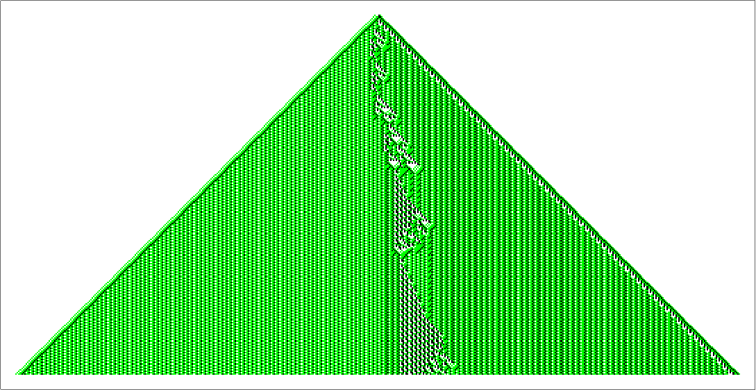
3-color Rule 6244262337426. This was found by modifying a random initial rule, with only the condition that the background remains white.
ArrayPlot[CellularAutomaton[
  {6244262337426, 3, 1}, (* Rule *)
  {{1, 1, 0, 0, 1, 1, 0, 2}, 0}, (* Initial Condition - the interesting one *)
  350], (* Number of Steps *)
 ColorRules -> {0 -> White, 1 -> Green, 2 -> Black}] (* Coloring *)
Most small initial conditions get repetitive.
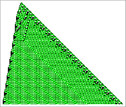
However, I've found {1,1,0,0,1,1,0,2} is chaotic for at least 8000 steps.
3-color Rule 6613854010095. Just as before, this was found by modifying a random rule.
ArrayPlot[CellularAutomaton[
          {6613854010095, 3, 1}, (* Rule *)
          {{1, 0, 0, 2, 1}, 0}, (* Initial Condition - the interesting one *)
          350], (* Number of Steps *)
         ColorRules -> {0 -> White, 1 -> Green, 2 -> Black}] (* Coloring *)
As before, many small initial conditions do not generate anything interesting, however the initial condition {1,0,0,2,1} yields interesting computation:
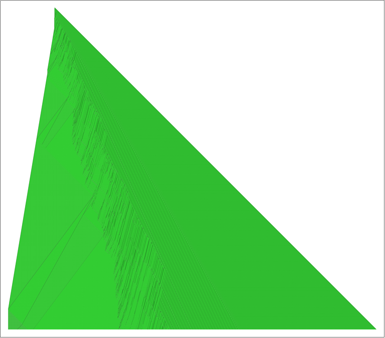
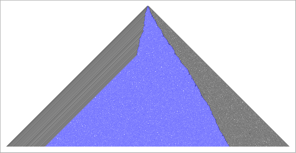
I've got many more examples, however less organized. I'll close out with this one though. This wasn't started from a random rule, but I was trying "artistically multiply" Rule 30 against its reverse using this same calibration method and some intuition, favoring randomness on the black left-edge (that might be a whole other conversation unto itself). I got something a bit more interesting than I expected. 3-color rule number 892507546128, with various initial conditions:
ArrayPlot[CellularAutomaton[
  {892507546128, 3}, (* Rule *)
  {RandomInteger[2, 17], 0}, (* Initial Condition *)
  750], (* Steps *)
 ColorRules -> {0 -> White, 1 -> Blue, 2 -> Black}] (* Coloring *)
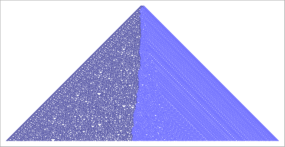
This has very different global behavior depending on initial conditions, combined with all the chaos and order you'd expect out of something based on Rule 30. The remaining images are of this rule, with varying random (and unfortunately unsaved except for the images) initial conditions:
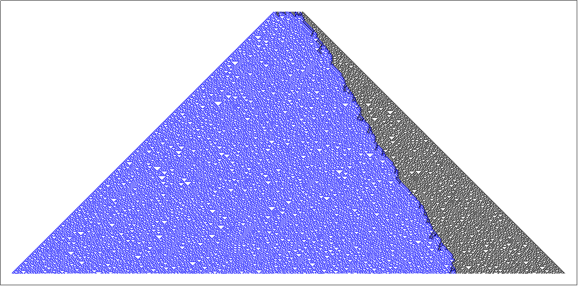 There's randomness on both sides, this I expected would always be the case.
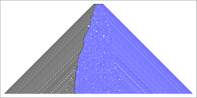
There's significant order on both sides. This I didn't expect at all. It also looks like chaos spontaneously begins on the left.
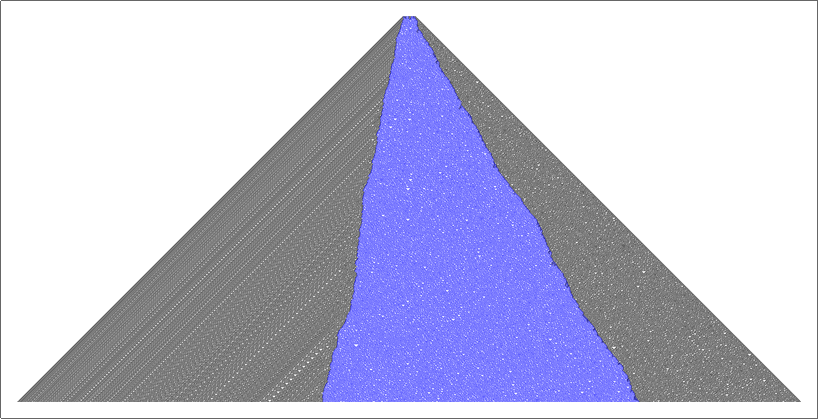
 These only confused me further, especially the sudden dog-earing of the blue section to the left.
 This doesn't even look like the same rule. Blue and black are mixed on the left. Per my notebook it's the same rule as above.
I mostly follow cellular automaton recreationally -- I haven't been reading any formal papers about it. I'm not sure if looking at CA in terms of directionalized correlation and computation is new or studied. I'm also not sure if there are known methods for generating cool cellular automata. I'd expect this is nothing new I've stumbled on, but honestly, I'm not seeing enough CA art that would hint at methods for making novel CA, and part of me thinks at least that bit is new.
Feedback is welcome, especially if you know of specific disciplines, papers, or people that pertain to either of these ideas. Thanks!


