Hi Megan,

I'm not sure if I'm following you, but maybe this will help. We start with a random list of -1s and 1s. At each step we flip one of them randomly. If the flip increases the number of 1s then we keep it as our new state, otherwise we keep the old state. We stop when all of them are 1s.

The main function we will use is NestWhileList.The start state is simple.So is the continue test.The & is a short way to write functions (called pure functions). The # will be replaced with the list of 1s and -1s for the current state when the function is used. You can read more about how to use this short syntax here.

I'm going to use more pure function syntax and write them in a right-to-left manner to shorten the code for the step function as well. The input to our step function is the old state. First we want to make a list containing the old state and the potential new state where a random value has been multiplied by -1.Now I'll chain on another function for choosing between the two by prepending &@@. The & starts a new function and the @@ means I can refer to the old state as # and the new state as #2 in the new pure function. If the total of the new state is more than the total of the old state we'll keep the new one. Otherwise, we keep the old one and try again on the next step.Now we have our three arguments for NestWhileList and we can use MatrixPlot to visualize the results. Here is all of the code together.
Running the code gives something like this, which took 23 steps to reach the minimum energy state of all 1s.

It takes a long time to learn all of the commands in Mathematica.

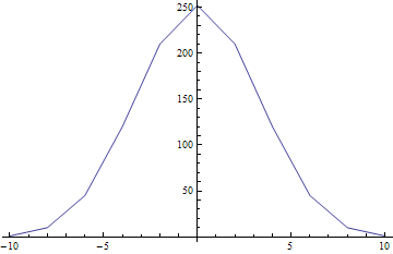
For the Boltzmann distribution do you want a plot of the number of states for each energy? Here's how to do that. Use Tuples to generate a list of all possible states. Then Map (/@) the command Total across the list to transform each state into its energy. Then Tally the number of times each energy appears and plot it.


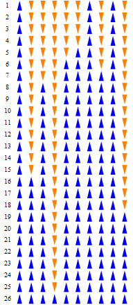
MatrixPlot does allow you to label the steps, but you can only choose the colors for the squares for each neutron state. It's pretty easy to just replace each 1 or -1 with an up or down arrow and show those in a GraphicsGrid though. Here's how to do that. You can use ReplaceAll (/.) with rules for 1 and -1 to replace each number with an arbitrary image. This uses small blue up arrows and orange down arrows.Then we can go to each row and Prepend a step number in front of it and then display the whole thing as a GraphicsGrid.Here is all of the code as one expression. You can triple-click on different parts to select the various subexpressions when reading it in a notebook.