In their article "Generation of view dependent models using free form deformation", Guy & Sela Gershon Elber coined the term "sqriancle"(SQuare, tRIANgle and cirCLE) as an object that looks like a square, a triangle or a circle when observed from different angles. A picture of the same object appeared in "Advances in Architectural Geometry 2010" edited by Cristiano Ceccato et al.
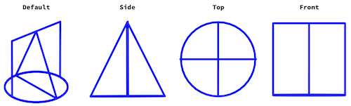
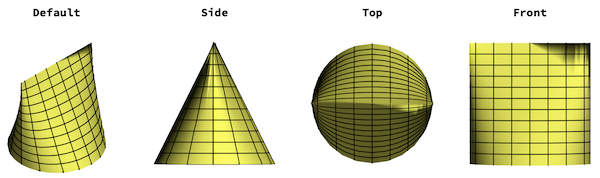
Let us see what this "view dependent object" looks like in Mathematica. Here is a ring-like object that could form the base of our sqriancle as it appears as a square, triangle or circle depending on the viewpoint.
Grid[{Style[#, Bold] & /@ {"Default", "Side", "Top", "Front"},
  Graphics3D[{{FaceForm[], EdgeForm[{AbsoluteThickness[4], Blue}],
       Cylinder[{{0, 0, 0}, {0, 0, .01}} 1]}, {Blue,
       AbsoluteThickness[4], Line[{{0, 1, 0}, {0, 0, 2}, {0, -1, 0}}],
        Line[{{-1, 0, 2}, {1, 0, 2}}], Line[{{1, 0, 0}, {1, 0, 2}}],
       Line[{{-1, 0, 0}, {-1, 0, 2}}]}}, Boxed -> False,
     ViewPoint -> #] & /@ {{30, 35, 25}, {50, 1, 0}, {0, 0,
     50}, {0, -50, 0}}}]
This shows the geometry of a sqriancle consisting of a unit circle, a unit square perpendicular to it along the diameter and a perpendicular triangle SQR with height h straddling the circle. A point P is on the contour of the triangle.
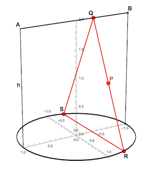
To create a volume with the 3 different views, we take the base SR of the triangle as a chord in the circle and thus dependent on x. A point P{x,y,z) on the boundary of the triangular cross section RSQ has the following coordinates:
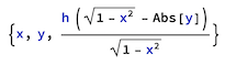
To compute the parametric surface, we convert the coordinates of P to polar form:
{x, y, (h (Sqrt[1 - x^2] - Abs[y]))/Sqrt[
    1 - x^2]} /. {x -> r Cos[phi], y -> r Sin[phi]} //
  Simplify // Rasterize
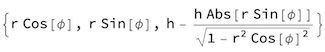
This is a function for the parametric coordinates of a point P on the sqriancle: r and phi are the polar coordinates of the projection of P in the x-y plane:
sqriancle[r_, phi_,
  h_ : 2] := {{r Cos[phi], r Sin[phi], 0.}, {r Cos[phi], r Sin[phi],
   h - (h Abs[r Sin[phi]])/Sqrt[1 - r^2 Cos[phi]^2]}}
Animate[ParametricPlot3D[
  sqriancle[r, phi], {phi, -Pi, 2 Pi}, {r, 0, 1},
  RegionFunction -> Function[x, x <= csx],
  BoundaryStyle -> Directive[Red, Thick],
  PlotStyle -> Lighter[Gray, .5], MeshFunctions -> {#1 &, #3 &},
  Mesh -> {{-.3, -.6, -.9, .9999, 0, .3, .6, .9}, 10},
  MeshStyle -> AbsoluteThickness[1], Boxed -> False,
  Axes -> False], {csx, 1., -1.}]
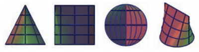
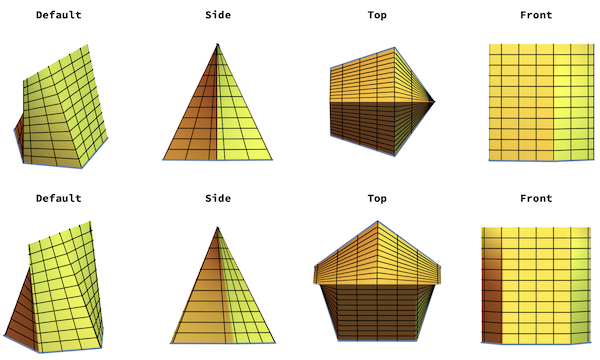
Here is how our sqriancle looks like if observed from viewpoints along the x-, y- and z-axes:
Grid[{Style[#, Bold] & /@ {"Default", "Side", "Top", "Front"},
  With[{h = 2.},
   ParametricPlot3D[sqriancle[r, phi], {phi, 0., 2 Pi}, {r, 0, 1},
      PlotPoints -> 25, PlotStyle -> Lighter[Yellow, .25],
      MeshFunctions -> {#1 &, #3 &},
      Mesh -> {{-.3, -.6, -.9, .9999, 0, .3, .6, .9}, 10},
      MeshStyle -> AbsoluteThickness[1], Boxed -> False,
      Axes -> False, ViewPoint -> #] & /@ {{35, 35, 35}, {50, 1,
      0}, {0, 0, 50}, {0, -50, 1}}]
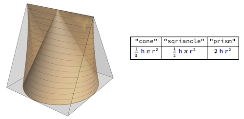
We can check that the sqriancle volume fits between a triangular prism and a cone:
Module[{co, sq, pr},
 co = Cone[{{0, 0, 0}, {0, 0, 2}}, .985];
 sq = First@
   ParametricPlot3D[sqriancle[r, phi], {phi, 0., 2 Pi}, {r, 0, 1.},
    PlotPoints -> 50, MeshFunctions -> {#3 &}];
 pr = Prism[{{-1, 0, 2}, {-1, 1, 0}, {-1, -1, 0},    {1., 0, 2}, {1.,
     1, 0}, {1., -1, 0}}];
 Row[{Graphics3D[{Opacity[.9], co, {Opacity[.5], sq}, Opacity[.3],
     pr}, Boxed -> False, Lighting -> "ThreePoint",
    ImageSize -> 300],
   Grid[{{"cone", "sqriancle", "prism"},
     Assuming[{h >= 0, r >= 0,
       Element[{r, h}, Reals]}, {Volume@
        Cone[{{0, 0, 0}, {0, 0, h}}, r],
       Integrate[h Sqrt[r^2 - x^2], {x, -r, r}],
       Volume@
        Prism[{{-r, 0, h}, {-r, r, 0}, {-r, -r, 0},    {r, 0, h}, {r,
           r, 0}, {r, -r, 0}}]}]}, Frame -> All]}]]
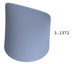
Using Volume on the discretized implicit region using h=2 and r=1, we approach the value above of Pi (3.1372) as the number of cells increases:
With[{h = 2.},
  reg = ImplicitRegion[
    0 <= z <= (h (Sqrt[1 - x^2] - Abs[y]))/Sqrt[
     1 - x^2], {{x, -1, 1}, {y, 0, 1}, z}]];
sqr = DiscretizeRegion[reg, AccuracyGoal -> 6, MaxCellMeasure -> .01]
Rasterize[Volume[sqr]]
We can make variations on the sqriancle in 3 ways, by changing the shape of either the circular z-axis cross section or the square or triangular cross sections of the y-and x-axes. We could e.g. use different regular polygons as alternative z-axis cross sections using the parametric. Here are two sets of views with a square bottom with 2 different rotation angles [Alpha] :
poly[t_, t0_, n_] :=
 Cos[Pi/n] Sec[(2 ArcTan[Cot[1/2 n (t - t0)]])/n] {Cos[t], Sin[t]}
ParallelTable[
 Module[{n = 4, sol},
  fits =
   Quiet[
    Table[{t0, FindMaxValue[Last[poly[t, t0, n]], t]}, {t0, 0, 2 Pi,
      Pi/16}]];
  sol[t_] :=
   Normal[
    Quiet[
     First[
      Solve[{x, y, z} \[Element]
        Line[{{First[poly[t, alpha, n]], 0, 2},
          Insert[poly[t, alpha, n], 0., -1]}], {x, y}]]]];
  Grid[{(Style[#1, Bold] &) /@ {"Default", "Side", "Top", "Front"},
    ParallelMap[
     Graphics3D[{{First[
          ParametricPlot3D[{x, y, z} /. sol[s], {s, 0, 2 Pi}, {z, 0,
            2}, PlotStyle -> Lighter[Yellow, .25],
           MeshFunctions -> {#1 &, #3 &},
           Mesh -> {{-.3, -.6, -.9, .9999, 0, .3, .6, .9}, 10},
           MeshStyle -> AbsoluteThickness[1],
           PlotRange -> {{-1, 1}, {-1, 1}, {0, 2}}]]},
        First[
         ParametricPlot3D[
          Insert[poly[phi, alpha, n], 0., -1], {phi, 0,
           2 Pi}]], {AbsoluteThickness[1]}}, Boxed -> False,
       PlotRange -> {{-1, 1}, {-1, 1}, {0, 2}},
       ViewAngle -> 1.5 Degree, Lighting -> "ThreePoint",
       ViewPoint -> #1] &, {{35, 35, 35}, {50, 1, 0}, {0, 0,
       50}, {0, -50, 1}}]}, Spacings -> 0]], {alpha, {.52, 1.55}}]
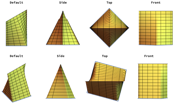
This is the same as above but with pentagonal bottoms rotated at different angles :
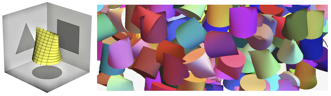
We take another look at our original sqriancle: Its shape appears as a triangular prism but it has a 22.5 % smaller volume. if it was used as an innovative shape for candy, it would mean less candy and sugar for the same apparent shape!
candy[col_, alpha_, ax_] :=
 Rotate[First@
   ParametricPlot3D[sqriancle[r, phi], {phi, -.01, 2 Pi}, {r, 0, 1},
    PlotPoints -> 50, PlotStyle -> col, Mesh -> False, Boxed -> False,
     Axes -> False], alpha, RotateRight[{0, 0, 1}, ax]]
Module[{c}, c = candy[Red, Pi/4, 2];
 Animate[
  Graphics3D[c, Boxed -> False,
   ViewVector ->
    RotationTransform[Pi/4, {1, -1, -1}]@{4 Sin[phi], 4 Cos[phi],
      8}], {{phi, 0}, 0, 2 Pi}]]

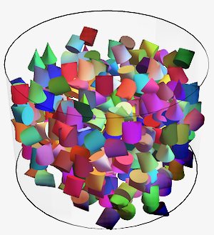
Here is a box full of it. Bon appetit!