SUPPLEMENTARY WOLFRAM MATERIALS for the ARTICLE:
Sergio Manzetti, Alexander Trounev (2021).
A Navier-Stokes model for Rogue wave simulation.
ResearchGate, Technical Report. https://www.researchgate.net/publication/354527324
ABSTRACT
Rogue waves are anomalous phenomena occurring over large sea bodies, where they are said appear out of nowhere and disappear without a trace. Simulations of rogue waves have been carried over the last 40 years, with several models published. In this paper we investigate the formation of rogue waves by two models: I. the Navier-Stokes equation where we take into account density and viscosity gradient on the air-water interface due to diffusion and II. a Korteveg de Vries-type model for quantum jumps which we developed earlier. We derive also a stable fluids algorithm which we use to compute nonlinear waves interaction produced by the wind. The results are discussed and compared.
This code solves problem of viscous incompressible flow with gravitational force in a rectangle with periodic boundary condition on the left and right side and with Dirichlet condition on the top and bottom side. In the initial condition fluid velocity is periodic wave, and density has unit step like distribution on the air/water interface. Some other application of this code has been discussed on https://mathematica.stackexchange.com/questions/246091/stable-fluids-code-for-electromagnetic-mixture-application
This model has been discussed in our report A Navier-Stokes model for Rogue wave simulation
Two phase model of air-water interface
Let us consider the system of equations describing nonlinear waves on the air-water interface. As it well known the air and the water can be considered as viscous incompressible fluids with density $\rho_a, \rho_w$, and dynamical viscosity $\mu_a, \mu_w$ consequently. Taking into account the gravity force and diffusion on the air-water interface, we have $$\nabla.\bf{u}=0\\ \frac{\partial \mathbf{u}}{\partial t}+(\mathbf{u}.\nabla)\mathbf{u}+\frac{\nabla P}{\rho_i}=\nu_i\nabla ^2\mathbf{u}+\mathbf{f}\\\ \frac{\partial \phi}{\partial t} +(\mathbf{u}.\nabla)\phi=\frac{\nu_i}{Sc_i}\nabla ^2\phi\\ $$ Here it is indicated $\rho_i, i=a,w $ - air and water density, $\mathbf{u}=(u_x,u_y)$ - flow velocity, $P$ - pressure; $\bf{f}$ - force acting on the volume of the air-water mixture; $\phi$ - the interface function describing the averaged density of the air-water mixture; $Sc_i$ - analog of the Schmidt number characterized water diffusion in the air and air diffusion in the water. Note that we considered averaged effect of mass transfer on the air-water interface including drops and bubbles. Let us define the Cartesian coordinate system so that the $y$ axis is directed against the direction of the gravitational acceleration vector and the $x$ axis is parallel to horizon. Let suppose that the water surface relief is described by the equation $y=r(t,x,y)$ - Figure 1. 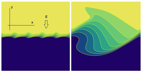
We set the boundary conditions for the flow parameters on the top and bottom part of the boundary layer and periodic boundary conditions by coordinate $x$ as follows:
$$ y=0: \mathbf{u}=0,\phi=\rho_w\\ y=H: \mathbf{u}=(U_0,0), \phi=\rho_a\\ \mathbf{u}(t,0,y)=\mathbf{u}(t,L,y)\\ \phi(t,0,y)=\phi(t,L,y). $$ Here $H$ is the height of the boundary layer,$U_0$ is the wind velocity, $L$ is the period of the wave tray. We assume that at the initial time the flow velocity and interface function are given by
$$ t=0, y<H/2:u_x = 0, u_y=V_0 \sin(2 \pi n x/L), \phi =\rho_w\\ t=0, y\ge H/2: u_x=U_0, u_y=V_0\sin (2 \pi n x/L), \phi =\rho_a\\ $$ This problem can be solved with using numerical methods and an appropriate turbulence model. We have used stable fluids algorithm (Stam1999, Stam 2000) to solve 2D Navier-Stokes equations and to simulate nonlinear waves interaction on the air-water interface with a given wind velocity on the top of the boundary layer. While in the standard gravity wave theory the air-water interface is considered mainly as a potential flow, in our approach we take into account velocity, viscosity and density gradients on the interface. Since air/water density ratio is about $10^{-3}$ we have some challenging numerical problem. To solve this problem we made some simplifications in the basic Navier-Stokes equations. First, we suppose that velocity is a continues field at $t>0$ so that flow in the water and flow in the air is an united flow continuously distributed from the bottom to the top and the periodic one in the $x$ direction. We neglect by the surface tension due to large scale of the waves. Therefore we don't need any boundary condition on the air-water interface. Second, at $t>0$ we introduce continues density as $\rho=\phi$ to compute velocity field on every step. Third, we use stable fluid algorithm in time in the very specific order described below.
Stable fluids algorithm
1) Solve advection equation with using boundary conditions, initial data from the previous step, and an implicit algorithm
$$ \frac{\partial \mathbf{u}_1}{\partial t}+(\mathbf{u}_1.\nabla) \bf{u}_1=0 $$
2) Solve diffusion equation with $\nu_i=\nu_i(\phi)$, initial data $\mathbf{u}_1$, boundary conditions and with using, for example, Gauss-Seidel relaxation algorithm
$$ \frac{\partial \mathbf {u}_2}{\partial t}-\nu_i \nabla^2 \mathbf{u}_2=0$$
here $$\nu_i(\phi)=\nu_w \phi ^k, k=-0.4029$$ for the air temperature of 20C.
3) Add force to the velocity field from the previous step as follows
$$ \mathbf{u}3=\mathbf{u}2+\mathbf{f} dt\ $$
To simulate force acting on the volume of air-water mixture we used approximation $$ f_y=-\frac{(\rho_w-\phi)(\phi-\rho_w/2)(\phi-\rho_a)}{\rho_w^2(\rho_w-\rho_a)Fr^2} $$ 4) Make projection step. Here we can use two models. First model is standard projection (Stam 1999) by solving Poison equation $$ t>0, \nabla^2 q=\nabla . \bf{u}_3\\ \bf{u}_4=\bf{u}_3-\nabla q $$ Note, that this step allows us to define divergent free velocity field.
5) Update velocity field $\bf{u}_4\longrightarrow \bf{u}_5$ with using boundary conditions.
6) Make diffusion step with interface function by solving diffusion equation with initial condition from the previous step, with boundary conditions, and with $\nu=\nu_i(\phi)/Sc$ as follows
$$ \frac{\partial \phi_1}{\partial t}-\nu \nabla^2 \phi_1=0 $$ 7) Make advection step by solving advection equation with initial data from step 6 with boundary conditions using an implicit algorithm (from step 1, for example),
$$ \frac{\partial \phi_2}{\partial t}+(\bf{u}_5.\nabla) \phi_2=0 $$ 8) Update interface function with boundary conditions.
9) Return to step 1 with updated velocity and interface function.
This algorithm can be also used in some different order, for example, in the beginning we can compute step 3 (Stam1999). Also we can make steps 6-8 first, and then compute velocity field with steps 1-5. The question about stability of the stable fluids algorithm not really solved yet. From our experience, we can't do arbitrary time step, but $dt$ is limiting by the grid size as usual for more precise computation. In our computations we have used $dt=2/N$ for $N\times N$ grid. In general case the numerical solution depends on the Froude number $Fr=\frac{U_0}{\sqrt{g L}}$, Reynolds number $Re=\frac{U_0 L}{\nu_w}$, Schmidt number and number of waves in the initial data. In our computations we fixed the Froude number, so that we can put $H=L=1$. We also fixed the Reynolds number, therefore we can put $U_0=1.5, V_0=0.5$. The algorithm 1-9 has been implemented with FDM and compiled to C with using Mathematica 12.3.
Code to simulate air/water interface with $Re=10^4, Fr=1$
rhoWater20C = 1.027; nuW20C = 0.01007; rhoAir20C = 0.001204; nuA20C = 0.151;dif = 1/10000; pec = .1; U0 = 1.5; V0 = .5; dn0 = 0.997658; dn1 = 0.514102; kap = 1; n = 81; Fr = 1; F0 = 1; n1 = n + 1; sm = 600; r = 20; den =
 ConstantArray[dn1 (1 + dn0 Tanh[-kap Range[-n1/2, n1/2]]), n1];u0 = ConstantArray[0, {n1, n1}]; Do[
  u0[[i, j]] = U0 (1 + Tanh[kap (j - n1/2)])/2;, {i, n1}, {j, n1}];
 v0 = ConstantArray[0., {n1, n1}]; Do[
  v0[[i, j]] = V0 Sin[10 Pi (i - 1)/n];, {i, n1}, {j, n1}];periodic[n_, up_, ud_, ub_] :=
    Module[{bd = ub}, Do[bd[[1, i]] = .5 (bd[[n, i]] + bd[[2, i]]);
      bd[[n + 1, i]] = bd[[1, i]]; bd[[i, 1]] = ud;
      bd[[i, n + 1]] = up;, {i, 2, n}];
     bd[[1, 1]] = .5 (bd[[2, 1]] + bd[[1, 2]]);
     bd[[n + 1, n + 1]] = .5 (bd[[n, n + 1]] + bd[[n + 1, n]]);
     bd[[n + 1, 1]] = .5 (bd[[n, 1]] + bd[[n + 1, 2]]);
     bd[[1, n + 1]] = .5 (bd[[1, n]] + bd[[2, n + 1]]); bd];

  diffuse[n_, r_, a_, c_, c0_] :=
    Module[{c1 = c},
     Do[Do[Do[
         c1[[i, j]] = (c0[[i,
               j]] + (a/den[[i, j]]^.4029) (c1[[i - 1, j]] +
                 c1[[i + 1, j]] + c1[[i, j - 1]] +
                 c1[[i, j + 1]]))/(1 + 4 a/den[[i, j]]^.4029);, {j, 2,
          n}];, {i, 2, n}];
      Do[c1[[1, i]] = c1[[n, i]]; c1[[n + 1, i]] = c1[[2, i]];
       c1[[i, 1]] = c0[[i, 1]];
       c1[[i, n + 1]] = c0[[i, n + 1]];, {i, 2, n}];
      c1[[1, 1]] = .5 (c1[[2, 1]] + c1[[1, 2]]);
      c1[[n + 1, n + 1]] = .5 (c1[[n, n + 1]] + c1[[n + 1, n]]);
      c1[[n + 1, 1]] = .5 (c1[[n, 1]] + c1[[n + 1, 2]]);
      c1[[1, n + 1]] = .5 (c1[[1, n]] + c1[[2, n + 1]]);, {k, 0, r}];
     c1];

  advect[n_, d0_, u_, v_, dt_] :=
    Module[{x, y, d1, dt0, i0, i1, j0, j1, s0, s1, t0, t1},
     d1 = ConstantArray[0, {n + 1, n + 1}]; dt0 = dt n;
     Do[Do[x = i - dt0 u[[i, j]]; y = j - dt0 v[[i, j]];
        i0 = Which[x <= 1, 1, 1 < x < n, Floor[x], True, n];
        i1 = i0 + 1;
        j0 = Which[y <= 1, 1, 1 < y < n, Floor[y], True, n];
        j1 = j0 + 1; s1 = x - i0; s0 = 1 - s1; t1 = y - j0; t0 = 1 - t1;
        d1[[i, j]] =
         s0 (t0 d0[[i0, j0]] + t1 d0[[i0, j1]]) +
          s1 (t0 d0[[i1, j0]] + t1 d0[[i1, j1]]);, {j, 1, n + 1}];, {i,
       1, n + 1}]; d1];

  project[n_, r_, u0_, v0_, u_, v_] :=
    Module[{ux = u, vy = v, div, p},
     p = ConstantArray[0, {n + 1, n + 1}];
     div = ConstantArray[0, {n + 1, n + 1}];
     ux = ConstantArray[0, {n + 1, n + 1}];
     vy = ConstantArray[0, {n + 1, n + 1}];
     Do[div[[i,
         j]] = -.5/
          n (u0[[i + 1, j]] - u0[[i - 1, j]] + v0[[i, 1 + j]] -
           v0[[i, j - 1]]);, {i, 2, n}, {j, 2, n}];
     Do[Do[Do[
         p[[i, j]] = (div[[i,
               j]] + (p[[i - 1, j]] + p[[i + 1, j]] + p[[i, j - 1]] +
                p[[i, j + 1]]))/4;, {j, 2, n}], {i, 2, n}];, {k, 0, r}];
     Do[ux[[i, j]] = u0[[i, j]] - .5 n (p[[i + 1, j]] - p[[i - 1, j]]);
      vy[[i, j]] =
       v0[[i, j]] - .5 n (p[[i, j + 1]] - p[[i, j - 1]]);, {i, 2,
       n}, {j, 2, n}]; {ux, vy}];

  Fx[t_, x_, y_] := 0;
  Fy[t_, x_, y_] := -1/Fr^2;

  onestep[n_, step_, r_, a_, uin_, vin_, dt_, c_] :=
   Module[{u1, v1, f1, f2, u, v, u0, v0},
    f1 = ConstantArray[0, {n + 1, n + 1}];
    f2 = ConstantArray[0., {n + 1, n + 1}];
    u0 = ConstantArray[0., {n + 1, n + 1}];
    v0 = ConstantArray[0., {n + 1, n + 1}];
    u = ConstantArray[0., {n + 1, n + 1}];
    v = ConstantArray[0., {n + 1, n + 1}];
    u1 = ConstantArray[0., {n + 1, n + 1}];
    v1 = ConstantArray[0., {n + 1, n + 1}]; u0 = uin; v0 = vin; Do[
     f2[[i, j]] =
       1/Fr^2 (den[[i, j]] - rhoWater20C/2) (rhoWater20C -
          den[[i, j]]) (den[[i, j]] - rhoAir20C)/(rhoWater20C -
            rhoAir20C)/rhoWater20C^2;, {i, 2, n}, {j, 2, n}];
    v0 += f2 dt;
    u0 = advect[n, u0, u0, v0, dt]; v0 = advect[n, v0, u0, v0, dt];
    mnV = 0;
    u0 = periodic[n, U0, 0, u0]; v0 = periodic[n, mnV, mnV, v0];
    u0 = diffuse[n, r, a, c, u0]; v0 = diffuse[n, r, a, c, v0];
    u0 = periodic[n, U0, 0, u0]; v0 = periodic[n, mnV, mnV, v0];
    {u1, v1} = project[n, r, u0, v0, u, v];
    u0 = periodic[n, U0, 0, u1];
    v0 = periodic[n, mnV, mnV, v1]; {u0, v0}]

  cf = With[{cg = Compile`GetElement, hp = HoldPattern,
      dv = DownValues},
     Hold@Compile[{{u0argu, _Real, 2}, {v0argu, _Real,
               2}, {denargu, _Real,
               2}, {sm, _Integer}, {n, _Integer}, {r, _Integer}, dif,
              pec, F0},
             Module[{u0 = u0argu, v0 = v0argu, uu, vv, dd,
               den = denargu, c = Table[0., {n + 1}, {n + 1}],
               dt = 40./n^2, a, dnup = den[[1, n + 1]],
               dnd = den[[1, 1]]}, a = dt dif n n;
              uu = vv = dd = Table[0., {sm + 1}, {n + 1}, {n + 1}];
              Do[

               den = advect[n, den, u0, v0, dt];
               den = periodic[n, dnup, dnd, den];
               den = diffuse[n, r, a/pec, c, den];
               den = periodic[n, dnup, dnd, den];

               dd[[step + 1]] = den; {u0, v0} =
                onestep[n, step, r, a, u0, v0, dt, c];
               uu[[step + 1]] = u0;
               vv[[step + 1]] = v0;, {step, 0, sm}]; {uu, vv, dd}],
             CompilationTarget -> C, RuntimeOptions -> "Speed"] /.
           dv@onestep /.
          Flatten[dv /@ {Fx, Fy, advect, diffuse, periodic, project}] /.
         hp@ConstantArray[c_, {i_, j_}] :> Table[0., {i}, {j}] /.
        hp@Part[a__] :> cg[a] /. hp[cg[a__] = rhs_] :> (Part[a] = rhs) //
       ReleaseHold];
Visualization
rst = cf[u0, v0, den, sm, n, r, dif, pec, F0];Do[lstu[k] =
   Flatten[Table[{{(i - 1)/n, (j - 1)/n}, rst[[1, k, i, j]]}, {i,
      n1}, {j, n1}], 1];
  lstv[k] =
   Flatten[Table[{{(i - 1)/n, (j - 1)/n}, rst[[2, k, i, j]]}, {i,
      n1}, {j, n1}], 1];, {k, sm}];
Do[Uvel[i] = Interpolation[lstu[i], InterpolationOrder -> 3];, {i, 1,
   sm}];
Do[Vvel[i] = Interpolation[lstv[i], InterpolationOrder -> 3];, {i, 1,
  sm}]; Do[lst4[k] =
   Flatten[Table[{{(i - 1)/n, (j - 1)/n}, rst[[3, k, i, j]]}, {i,
      n1}, {j, n1}], 1];, {k, sm}];
Do[rh[k] = Interpolation[lst4[k], InterpolationOrder -> 3];, {k, sm}];{ContourPlot[Uvel[10][x, y], {x, 0, 1}, {y, 0, 1},
  ColorFunction -> "BlueGreenYellow", Frame -> False,
  PlotRange -> All, ImageSize -> Small, MaxRecursion -> 2,
  Contours -> 15, ContourStyle -> Yellow, PlotLegends -> Automatic],
 ContourPlot[Vvel[10][x, y], {x, 0, 1}, {y, 0, 1},
  ColorFunction -> "BlueGreenYellow", Frame -> False,
  PlotRange -> All, ImageSize -> Small, MaxRecursion -> 2,
  Contours -> 15, ContourStyle -> Yellow, PlotLegends -> Automatic],
 ContourPlot[1 - rh[10][x, y], {x, 0, 1}, {y, 0, 1},
  ColorFunction -> "BlueGreenYellow", Frame -> False,
  PlotRange -> All, ImageSize -> Small, MaxRecursion -> 2,
  Contours -> 15, ContourStyle -> Yellow, PlotLegends -> Automatic],
 ContourPlot[Uvel[sm][x, y], {x, 0, 1}, {y, 0, 1},
  ColorFunction -> "BlueGreenYellow", Frame -> False,
  PlotRange -> All, ImageSize -> Small, MaxRecursion -> 2,
  Contours -> 15, ContourStyle -> Yellow, PlotLegends -> Automatic],
 ContourPlot[Vvel[sm][x, y], {x, 0, 1}, {y, 0, 1},
  ColorFunction -> "BlueGreenYellow", Frame -> False,
  PlotRange -> All, ImageSize -> Small, MaxRecursion -> 2,
  Contours -> 15, ContourStyle -> Yellow, PlotLegends -> Automatic],
 ContourPlot[1 - rh[sm][x, y], {x, 0, 1}, {y, 0, 1},
  ColorFunction -> "BlueGreenYellow", Frame -> False,
  PlotRange -> All, ImageSize -> Small, MaxRecursion -> 2,
  Contours -> 8, ContourStyle -> Yellow, PlotLegends -> Automatic]}
In this Figure are shown velocity components $u_x$ (left), $u_y$ (middle) and 1- density (right) on step 10 (upper line) and on final step $sm=600$ 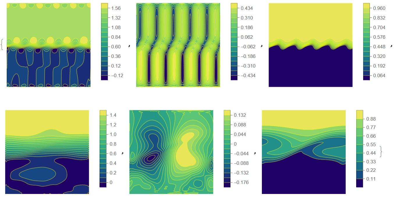
UPDATE
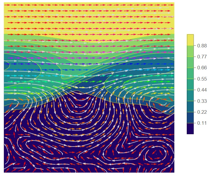
Next step is to animate wave transformation using interface function. We can show velocity field over density as follows
Show[ContourPlot[1 - rh[sm][x, y]/rhoWater20C, {x, 0, 1}, {y, 0, 1},
  PlotRange -> All, ColorFunction -> "BlueGreenYellow", Contours -> 8,
   ContourStyle -> Yellow, Frame -> False, PlotLegends -> Automatic],
 StreamPlot[{Uvel[sm][x, y], Vvel[sm][x, y]}, {x, 0, 1}, {y, 0, 1},
  PlotRange -> All, StreamColorFunction -> None, VectorPoints -> Fine,
   VectorColorFunction -> Hue, PlotLegends -> Automatic,
  StreamColorFunctionScaling -> True, StreamStyle -> LightGray]]
We can also compute frames for animation with using interface function
frames=Table[ContourPlot[1 - rh[i][x, y], {x, 0, 1}, {y, 0, 1},
  ColorFunction -> "BlueGreenYellow", Frame -> False,
  PlotRange -> All, ImageSize -> Small, MaxRecursion -> 2,
  Contours -> 8, ContourStyle -> Yellow, PlotLabel -> i], {i, 20, sm,
  20}]; Animate[frames]
References
Jos Stam. Stable fluids. In Computer Graphics Proceedings Annual Conference Series, Los Angeles, Aug. 3–8, 199.
Jos Stam. Interacting with smoke and fire in real time. Communications of the ACM, 43(7):77–83, July 2000.


