Message Boards Message Boards

Incorrect plot range when range is specified with unit

Posted 2 years ago

I was trying to make a square wave function that represents the pixel clock of our instrument.

PixelClock[pixelTime_, gapTime_] := 
 Piecewise[{{1, Mod[#, pixelTime] < (pixelTime - gapTime)}}, 0] &

I would prefer it can produce a function that takes time quantity as input, for example:

pc1 = PixelClock[Quantity[20, "Microseconds"], 
  Quantity[2, "Microseconds"]]

Running it with 1-100 microseconds as a list gives the expected answer.

pc1[Quantity[#, "Microseconds"]] & /@ Range[100]

Out[3]= {1, 1, 1, 1, 1, 1, 1, 1, 1, 1, 1, 1, 1, 1, 1, 1, 1, 0, 0, 1, \
1, 1, 1, 1, 1, 1, 1, 1, 1, 1, 1, 1, 1, 1, 1, 1, 1, 0, 0, 1, 1, 1, 1, \
1, 1, 1, 1, 1, 1, 1, 1, 1, 1, 1, 1, 1, 1, 0, 0, 1, 1, 1, 1, 1, 1, 1, \
1, 1, 1, 1, 1, 1, 1, 1, 1, 1, 1, 0, 0, 1, 1, 1, 1, 1, 1, 1, 1, 1, 1, \
1, 1, 1, 1, 1, 1, 1, 1, 0, 0, 1}

However, when I try to plot it, things get strange. enter image description here

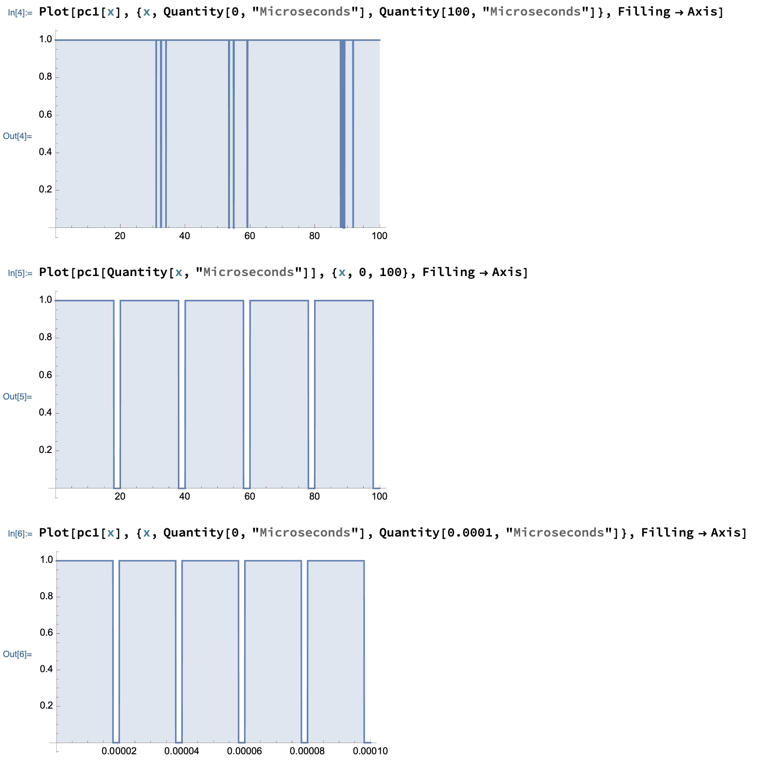
I would expect the first and the second plots to be equivalent. But they are not... I then realized if I reduce the value from 100 to 0.0001, the plot would look "correct" but is in fact using the wrong range. Is this a bug?

POSTED BY: Chen Huang
3 Replies

In case you're interested...

Square wave is kind of boring function to me, honest opinion, but they love it in the tech sector and the lab. I asked my dad about your question and he said it could be a 555 timer. However, in next gen on a rasbperry pi somewhere, there would need to be more complicated functions. Thank you too.

POSTED BY: Brad Klee

I checked on cloud, and found that yes this looks like a bug, not necessarily limited to one plot function. I also tried parametric plotting:

(*As clear as clear Space!*)
PCF = Quantity[PixelClock[Quantity[20, "Microseconds"], 
   Quantity[1, "Microseconds"]][#],"Volts"]&;
ParametricPlot[{Quantity[t, "Microseconds"], 
PCF@Quantity[t, "Microseconds"]}, {t, 0, 40},
Axes->False]

Documentation for plot explicitly allows quantity. No reason that parametric plot should behave any differently with input {t,F[t]}. The returns I got from that call was blank? Nice find, but my preference for simplicity would just always leave the plot parameter dimensionless, as it is in V.I. Arnold's math phys. theory. Here's another way to write the function & graph, assuming channel saturation at 1V:

PCF2 = ReplaceAll[Plus[SquareWave[{0, 1}, #/20],
     SquareWave[{1, 0}, #/20 + 2/20]], x_ /; x > 1 :> 1] &;
ParametricPlot[{t, PCF2[t]}, {t, 0, 50}, AxesLabel -> {"ms", "V"}]
Plot[PCF2[t], {t, 0, 50}, AxesLabel -> {"ms", "V"}]

outputs

The parametric plot is much more concerning, because I would think that expression is closer to what the output of an oscilloscope looks like (except without knobs to cycle units). Quantities are useful when doing conversions, but even then, my preferred method doesn't work in WL, for example:

Convert["Seconds,", "Milliseconds", val_] := Times[val,
  Divide[Quantity[1000, "Milliseconds"],
   Quantity[1, "Seconds"]]]
Convert["Seconds,", "Milliseconds", Quantity[1, "Seconds"]]
Out[]:=1s
POSTED BY: Brad Klee
Posted 2 years ago

Thanks very much for confirming the issue. I will report this to the WL support.

I don't mind keep the plot dimensionless in most cases. But for this one, it is not uncommon to have values that differ by a few orders of magnitude, so having the ability to just use the most convenient unit is ideal.

In case you're interested, while I was googling about this issue I've found another neat solution for generating this type of waves: https://mathematica.stackexchange.com/questions/7748/how-to-create-a-rectangle-wave-duty-cycle-ne-50#comment22019_7750

POSTED BY: Chen Huang
Reply to this discussion
Community posts can be styled and formatted using the Markdown syntax.
Reply Preview
Attachments
Remove
or Discard

Group Abstract Group Abstract