I've been thinking about what it would take to make a generically optimal autodiff engine, sorely missing right now and it comes down to einsum optimization, a well studied problem.
To see why you need an einsum optimizer, consider differentiating $F(x)=f(g(h(x)))$. Using chain rule we can write the derivative as the product of intermediate Jacobian matrices. $$\partial F = \partial f \cdot \partial g \cdot \partial h$$
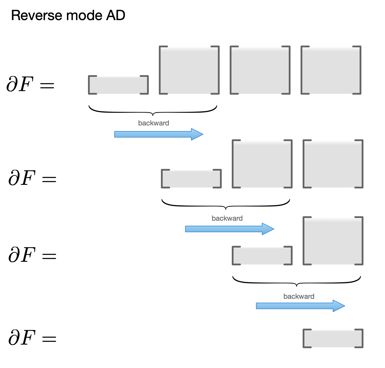
The optimal order of computing this matrix product depends on shapes of constituent matrices. This is the well known matrix-chain problem. For neural network applications, $f$ is the "loss" with scalar output, while intermediate results are high-dimensional, so the matrix product starts with short Jacobian matrix followed by square'ish matrices, and the optimal order is "left-to-right", aka "reverse mode differentiation." The process of doing vector/matrix product is known as the "backward" step in autodiff systems.
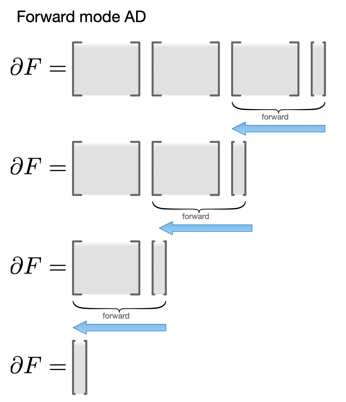
For different set of matrix shapes, you may need a different order. For instance, if output of $F$ is high-dimensional but $x$ is scalar, it's faster to multiply your Jacobians in the opposite order:
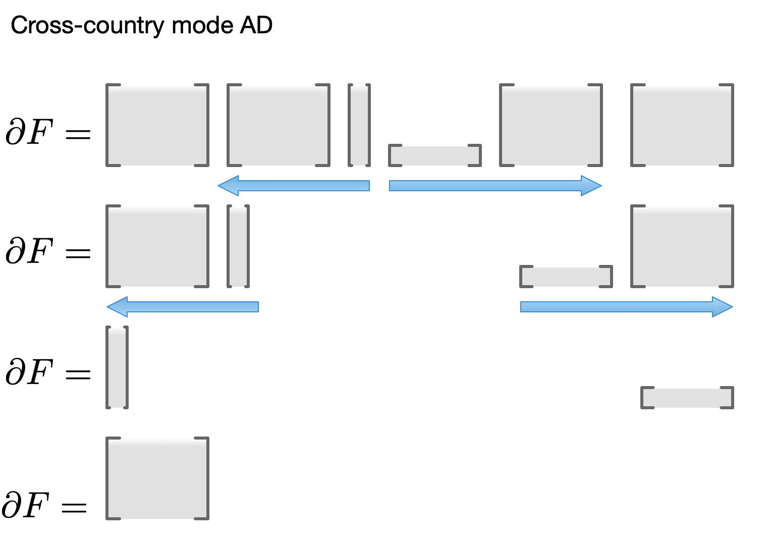
Or, suppose both input and output of $F$ are high-dimensional, but an intermediate result is low-dimensional. Then an optimal order would go outwards in both directions, followed by an outer product in the last step:
Commonly occuring orders have names in autodiff literature -- forward, reverse, mixed, cross-country, but there's really an infinity of such orders. You can solve this problem more generally by treating it as a problem of finding an optimal contraction order. This is a well-known problem in graph theory literature, corresponding to the problem of finding optimal triangulation in the case of chain (see David Eppstein's notes).
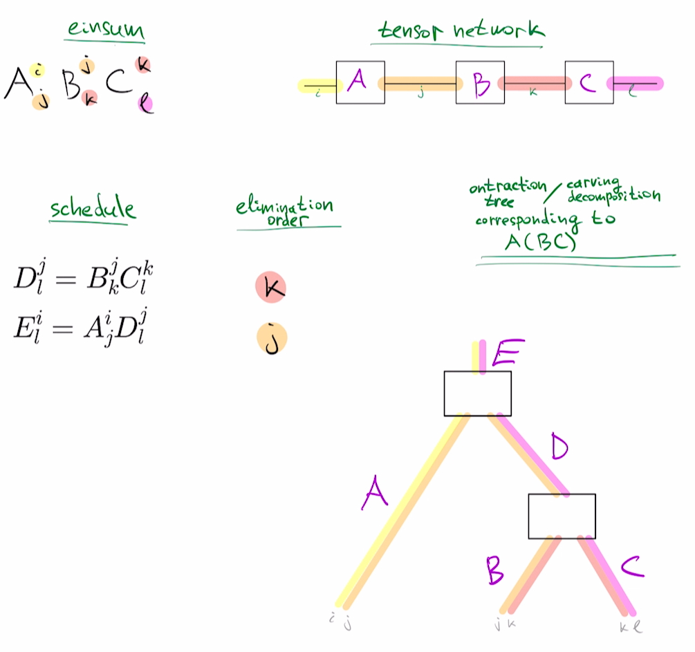
To see the connection of matrix chain problem to tensor networks, note that a product of matrices ABC can be written as a tensor network by using Einstein's summation notation:
$$ABC=A^{i}_j B^j_k C^k_l$$
This corresponds to a chain-structured tensor network below: 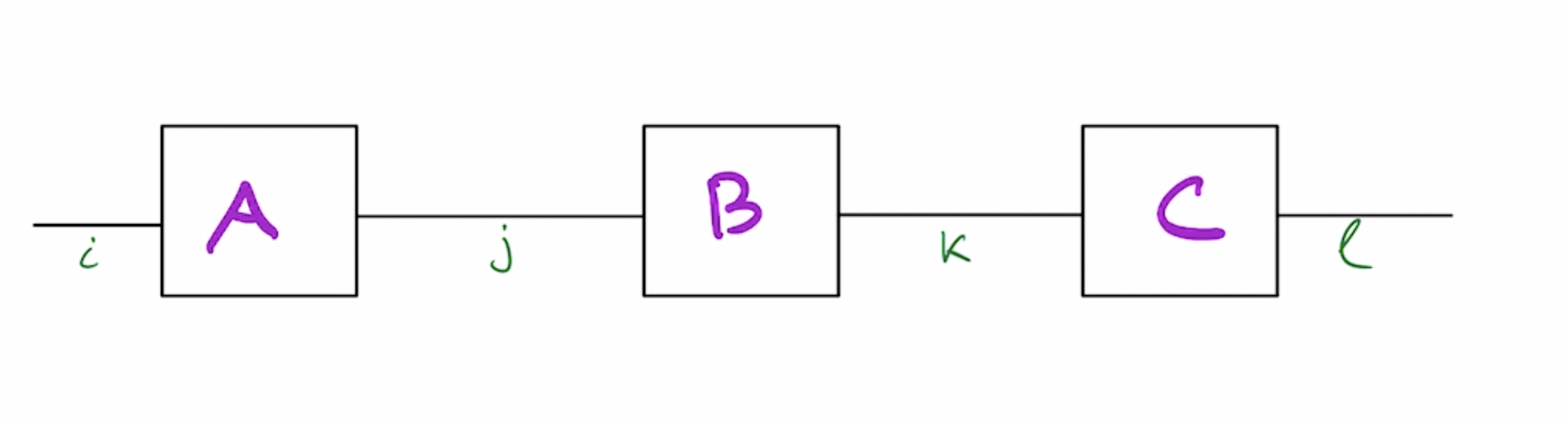
There are different orders in which you can perform the matrix multiplication. For instance, you could do $A(BC)$ or $(AB)C$. A parenthesization like $A(BC)$ is a hierarchical clusterings of tensors $A,B,C$ which is known as the "carving decomposition" of the tensor network graph, and it provides an order of computing the result, known as the "elimination order". For instance, computing $A(BC)$ corresponds to eliminating $k$, then $j$ and corresponding carving decomposition can be visualized below:
For a general tensor network, the problem of optimal elimination corresponds to the problem of finding the optimal carving decomposition. If individual tensor dimensions are all very large, this is equivalent to finding minimum-width carving decomposition, which is also equivalent to finding a tree embedding that minimizes edge congestion for the tensor network graph.
For instance, for the contraction problem in the paper, to compute $K=A_{ij} B_{ml}^i C_o^l D_k^j E_n^{km}F^{no}$, elimination sequence $j,m,i,k,o,l,n$ corresponds to the contraction tree below, giving edge congestion of $4$, because of the four colored bands along the edge $H$, indicating that it is a rank-4 tensor.
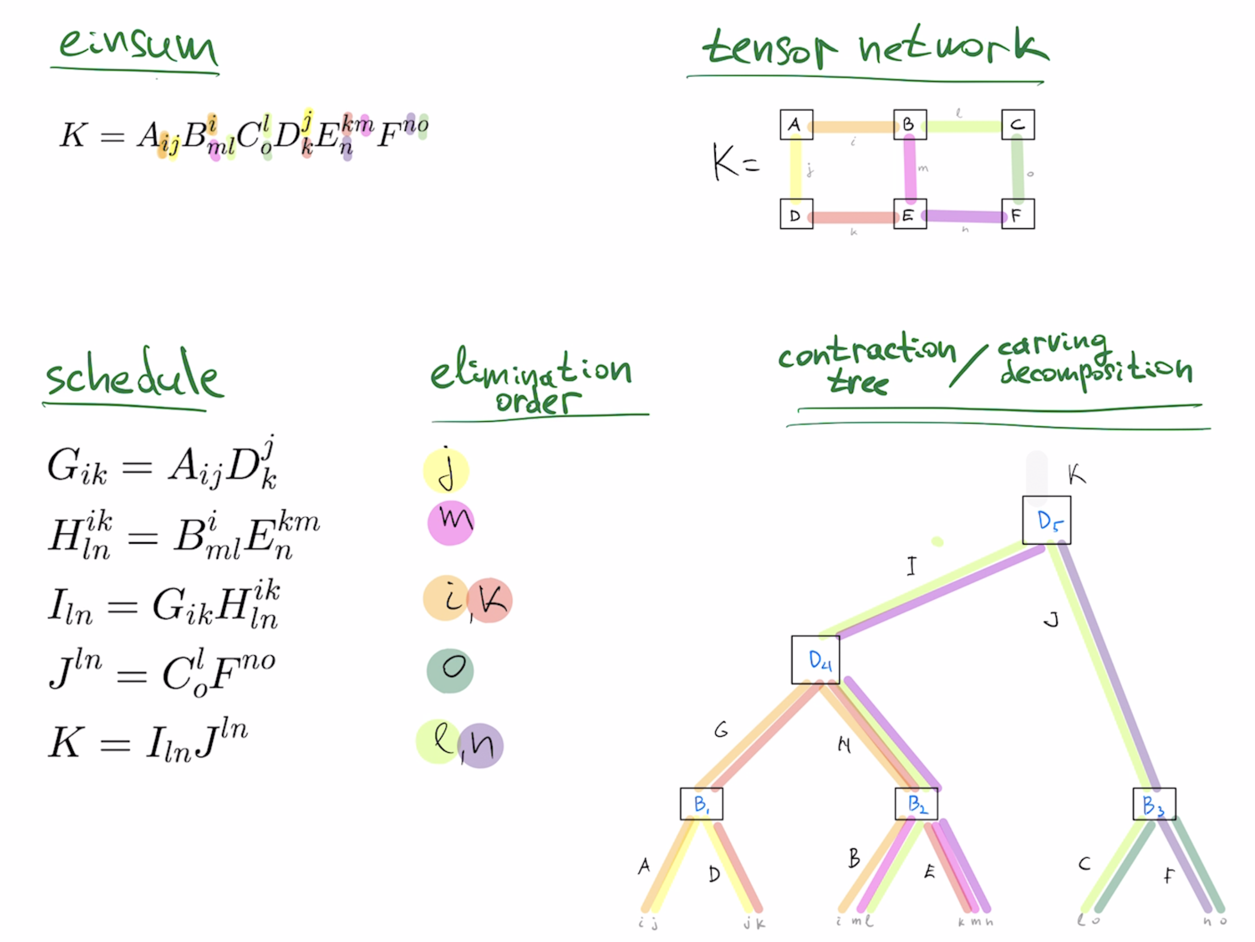
The rank of largest intermediate tensor in the minimum-width contraction schedule is the "carving-width" of the graph, so if Mathematica's GraphData supported "Carvingwidth" property, we could see "4" as the result of GraphData[{"Grid",{3,2}}, "Carvingwidth"] . Carving width of planar graphs as well as their minimum width carving decomposition can be computed in $O(n^3)$ time using the Ratcatcher algorithm.
For the simpler case of chain structured tensor network, we can solve the problem by using opt_einsum package which can handle general tensor networks. The package has been targeted for large tensor networks occurring in quantum mechanics, so solutions it gives for small tensor networks are sometimes suboptimal.
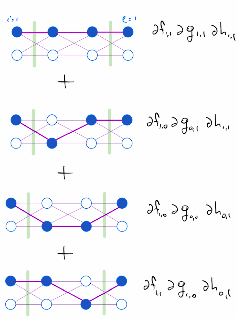
Another way to approach this problem is to view it as a sum over weighted paths problem. Suppose our functions $f,g,h$ all have 2 dimensional inputs and outputs. Given that $F(x)=f(g(h(x)))$, $\partial F$ is the matrix product $\partial f \cdot \partial g \cdot \partial h$, visualized pictorially below 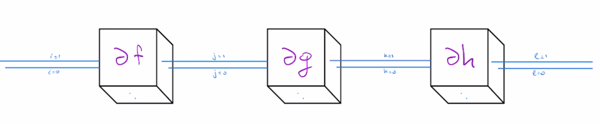
Derivative of this composition reduces to computing the sum over all paths for a fixed starting point and ending point, where weight of each path is the product of weights of individual edges, with edge weights corresponding to partial derivatives of intermediate functions $f,g,h$
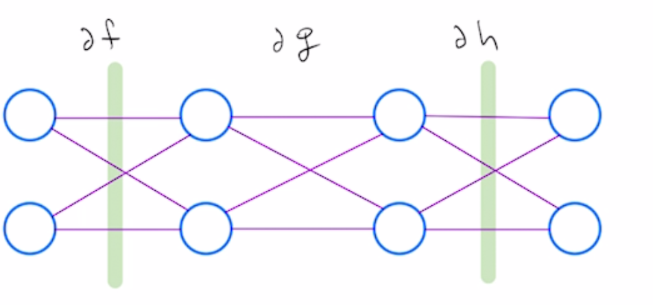
For instance, $\partial F_{1,1}$ is the sum over the following 4 paths, all with endpoints at $i=1$ and $l=1$:
Hence, an einsum optimizer provides an efficient way to solve the "sum over weighted paths" problem by reusing intermediate results optimally.
Classical solution to this problem is a dynamic programming algorithm with $O(n^3)$ scaling, but there's an $O(n^2)$ algorithm described here, with a Mathematica implementation here.
For more general automatic differentiation, you need an einsum optimizer that can optimize computation of a sum of tensor networks.
To see why, consider differentiating the following function:
$$F(x)=f(g(h(x))+h(x))$$
This addition corresponds to a "skip-connection", which is popular in neural network design. You "skip" an application of $g$ in the second term. As the sum of weighted paths, the derivative of $F$ can be visualized below: 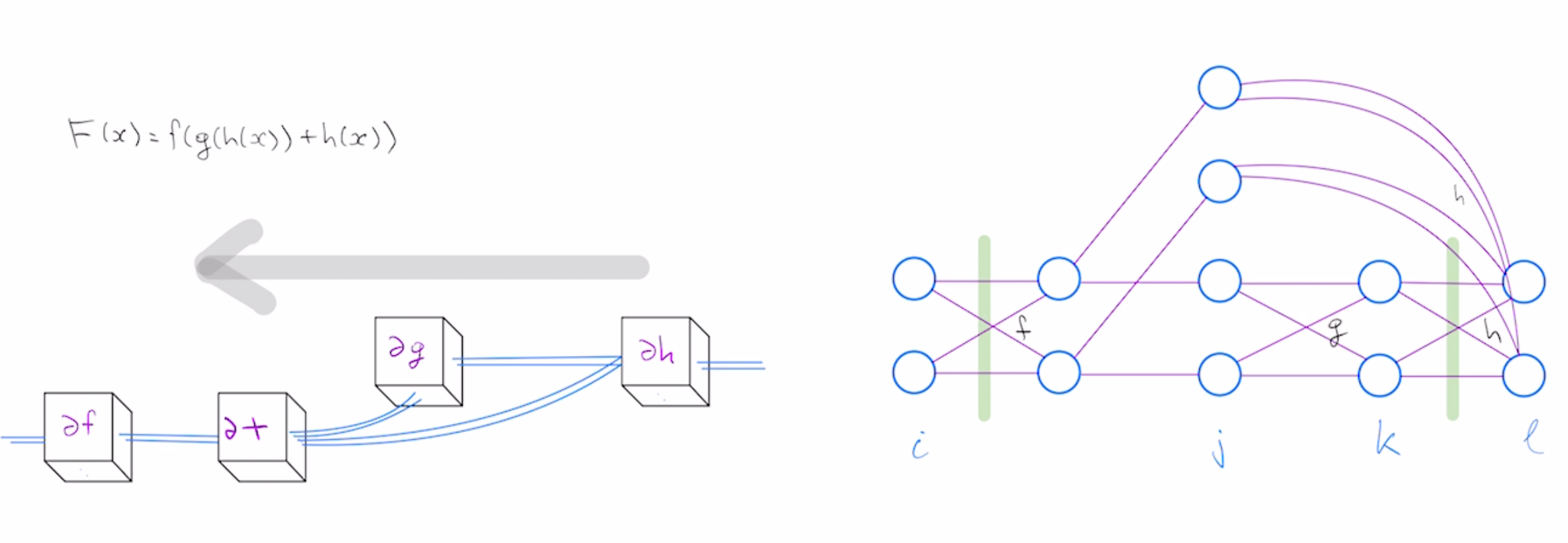
This doesn't neatly fit into tensor network notation, however, it does reduce to the sum of two tensor networks:
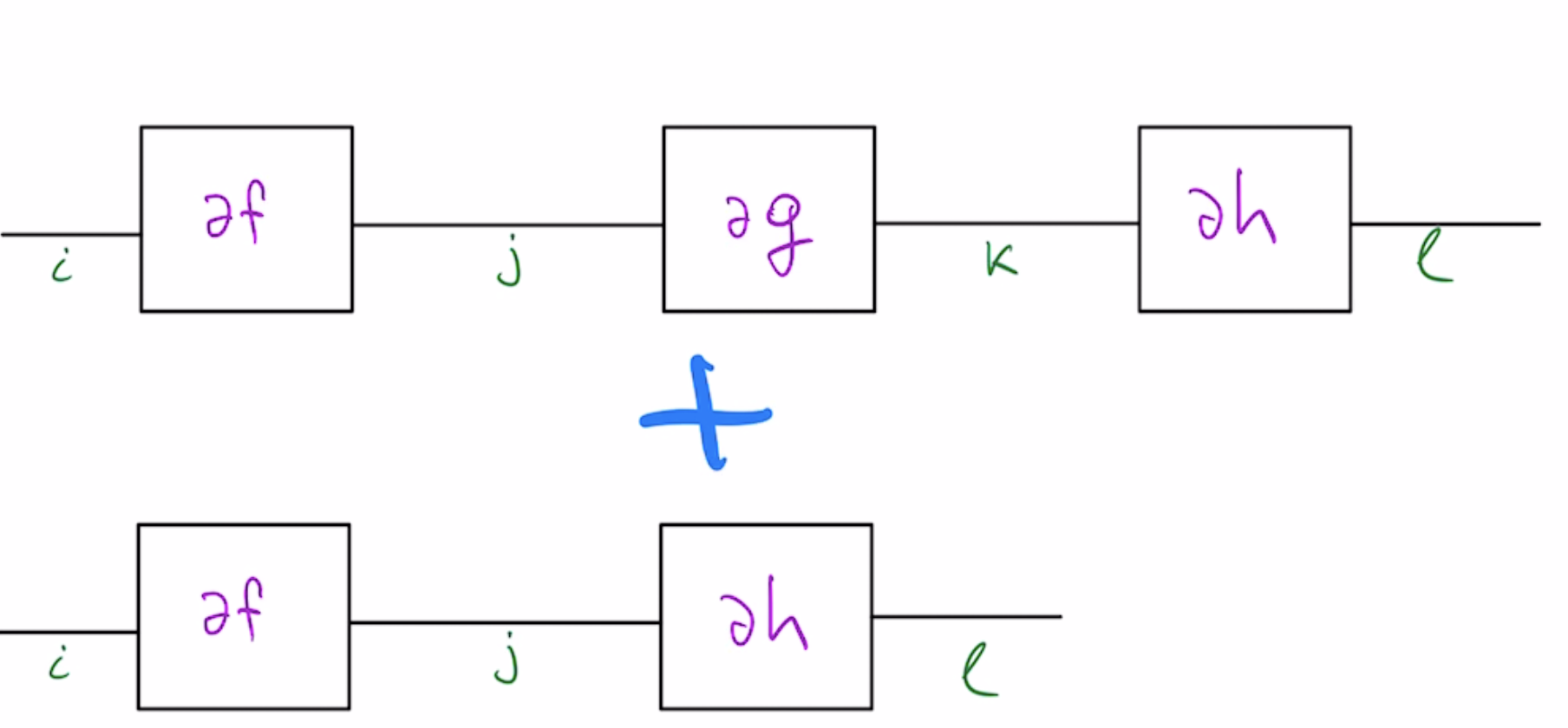
These tensor networks have sub-chains in common, so an optimal computation schedule may reuse intermediate across two networks. The problem of optimal AD schedule for skip connections is described in more detail here.
Another case where you need to optimize a sum of tensor networks is when computing Hessian-vector product of simple function composition. This comes up in Chemistry problems, see discussion here.
For a composition $F(x)=h4(h3(h2(h1(x))))$ with scalar-valued $h4$, the Hessian vector product of $F$ with vector $v$ is the following sum of tensor networks:
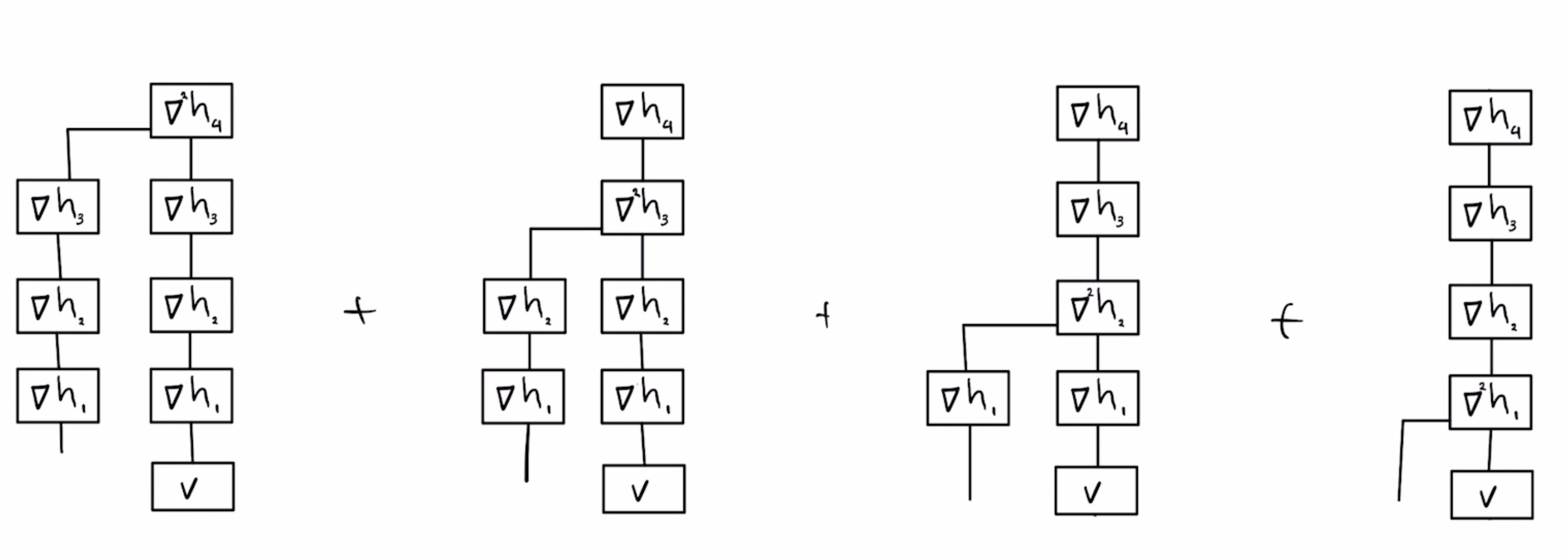
We can visually inspect this sum to manually come up with a schedule for computing Hessian-vector product $\partial^2 F \cdot h$ that takes about the same time as computing the derivative $\partial F$ 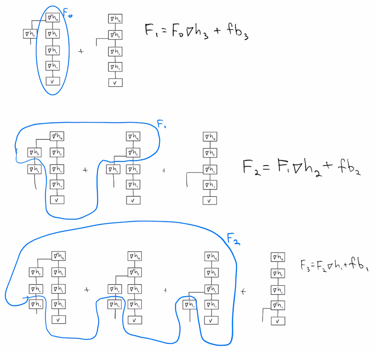
Here's a notebook (see below) implementing this schedule to compute Hessian-vector product of composition of functions $h_1, h_2, \ldots, h_n$ in Mathematica. It gives the same result as the built-in D[] functionality, but much faster.
The main parts of implementation are below. First define compute Jacobians and Hessians of intermediate functions stored in a list hs:
(* derivative of i'th layer *)
dh[i_] := (
   vars = xs[[i]];
   D[hs[[i]][vars], {vars, 1}] /. Thread[vars -> a[i - 1]]
   );

(* Hessian of i'th layer *)
d2h[i_] := (
   vars = xs[[i]];
   D[hs[[i]][vars], {vars, 2}] /. Thread[vars -> a[i - 1]]
   );
Now define the recursions to compute the schedule above. In autodiff literature, this would be called "foward-on-backward" schedule:
(* Forward AD, f[i]=dh[i]....dh[1].v *)
f[0] = v0;
f[i_?Positive] := dh[i] . f[i - 1];

(* Backward AD, *)
b[0] = {};
b[i_?Positive] := dot[b[i - 1], dh[n - i + 1]];

(* Activations *)
a[0] := x0;
a[i_?Positive] := h[i][a[i - 1]];
Now define the step that combines previous quantities into Hessian-vector products:
fb[i_] := dot[b[n - i], d2h[i]] . f[i - 1];

F[0] = fb[n];
F[i_?Positive] := F[i - 1] . dh[n - i] + fb[n - i];
After hours of manually debugging mismatched indices, it was especially satisfying to be able to write the following and have it work:
hess=D[H,{x0,2}];
Assert[Reduce[F[n-1]==hess.v0]];
Another example of derivative quantity that an autodiff engine should support is the Hessian trace. For the problem above, it can be written as the following sum of tensor networks:
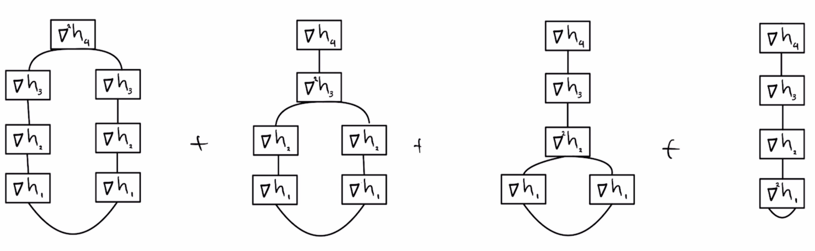 Boxes corresponding to $\nabla h_i$ are intermediate Jacobian matrices, while entries like $\nabla^2 h_i$ are Hessian tensors. They are potentially large, but for common intermediate functions occurring in neural networks Hessians tend to be structured -- 0, rank-1, diagonal or a combination of the two. For instance, for ReLU neural network with linear/convolutional layers, the only component with a non-zero Hessian is the $h4$ loss function, hence Hessian trace reduces to a loop tensor network
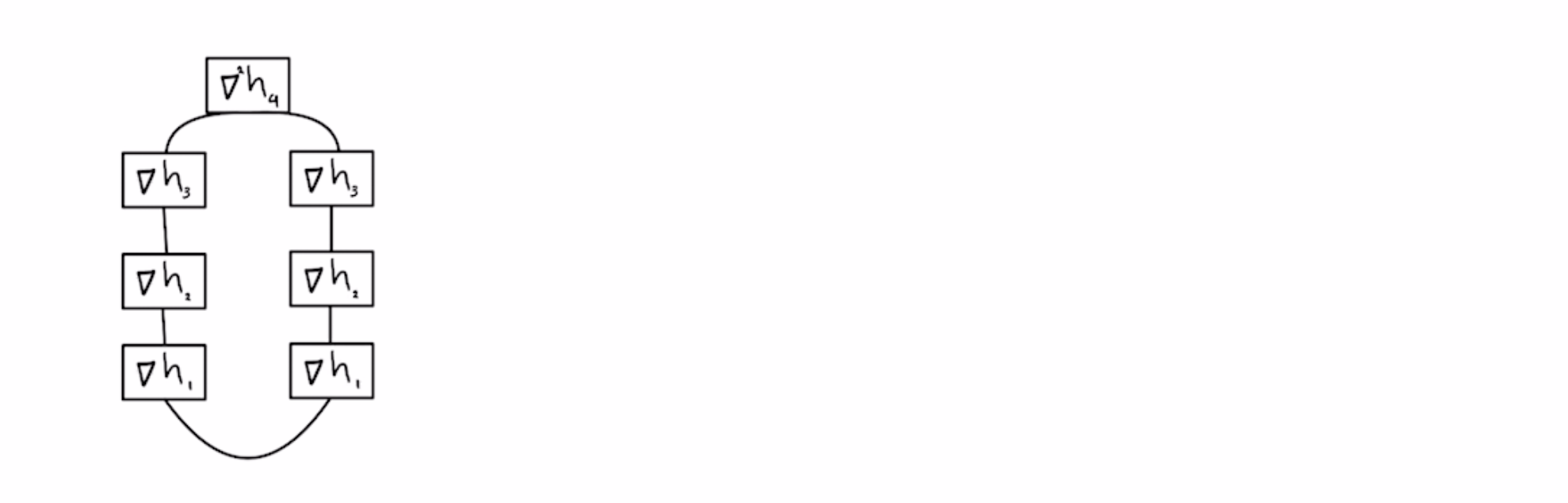
Furthermore, if the loss function $h4$ is the cross entropy loss, its Hessian corresponds to a difference of diagonal and rank-1 matrices, so the trace can be written as the following difference of two tensor networks
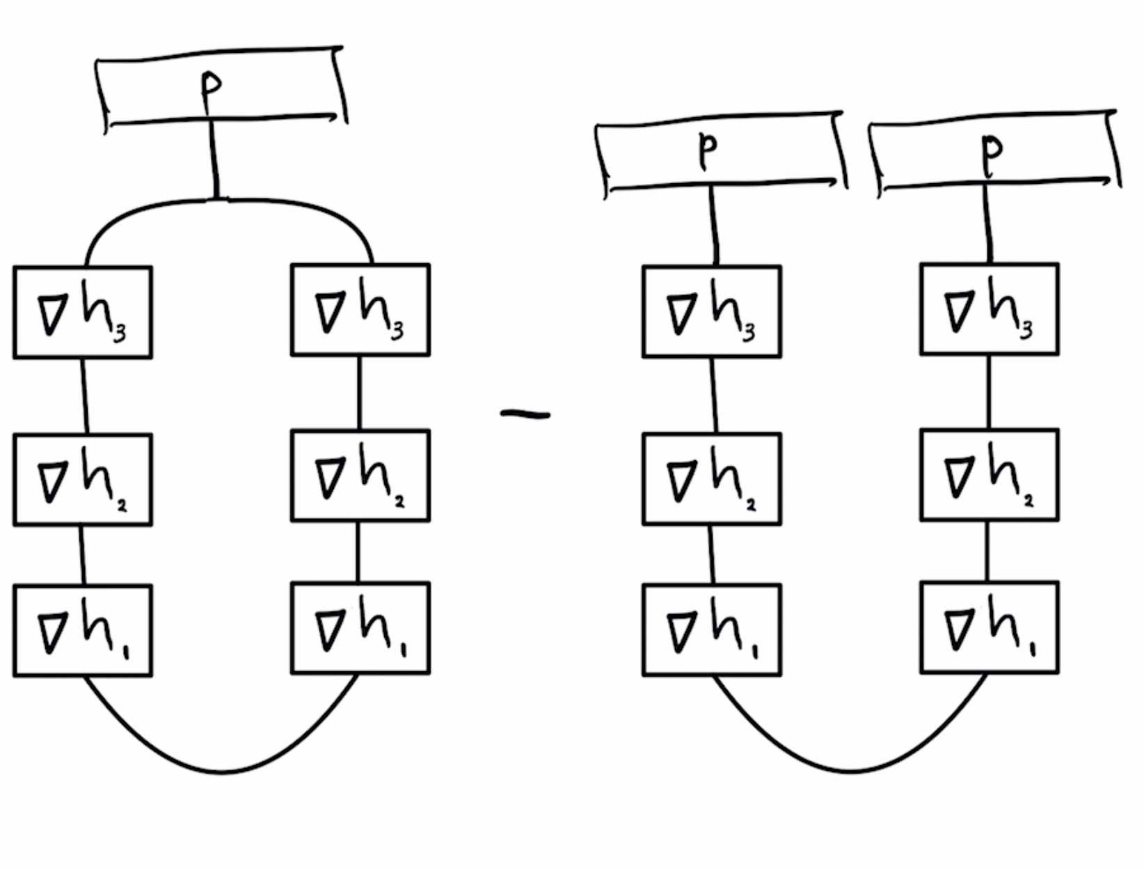
The 3 way hyper-edge connected to p in the diagram above is called the "COPY-tensor" in Quantum Tensor Network literature (see Biamonte's excellent notes), but in einsum notation it's just an index that occurs in 3 factors, np.einsum("i,ik,il->kl", p, h3, h3)
In addition to einsum notation, the expression above can be written in matrix notation as follows $$\text{tr} \nabla^2F=\|\text{diag}(\sqrt{p}) \nabla h_3 \nabla h_2 \nabla h_1\|_F^2 - p'\nabla h_3 \nabla h_2 \nabla h_1 \nabla h_1' \nabla h_2' \nabla h_3' p $$
Carl Woll has a nice package for converting einsums to matrix notation, it could probably be extended to also work for this case.
The problem of optimally contracting a general tensor network is hard, and people who implemented packages like opt_einsum and Cotengra mainly tried to approximate optimal solutions for large problems, like validating Google's Sycamore quantum supremacy result.
However, tensor networks occuring up in automatic differentiation tasks are much easier than general tensor networks:
- all examples above are planar, for which a schedule within a factor of $n*d$ of optimal cost can be found in $O(n^3)$ time using Ratcatcher algorithm, $n$ is the number of tensors and $d$ is the largest bond dimension, (discussion)
- furthermore, all examples above are "series-parallel" graphs, treewidth=2
- furthermore, some examples are trees, for which a polynomial algorithm to obtain an optimal contraction algorithm has been described here
A practically interesting solution would be to create an einsum optimizer that can do one or more of the following:
- compute optimal contraction schedule for a tree-structured tensor network, allowing hyper-edges (detailed example here)
- compute optimal contraction schedule for a series-parallel tensor network
- compute optimal computation schedule for a sum of chain tensor networks (especially sums corresponding to derivatives of compositions with skip connections)
- compute optimal computation schedule for sum of tree tensor networks
- compute optimal computation schedule for a sum of series-parallel tensor networks
A tool that can do all of these efficiently for networks with 2-20 tensors would cover most autodiff applications that make sense to attempt in Mathematica.


