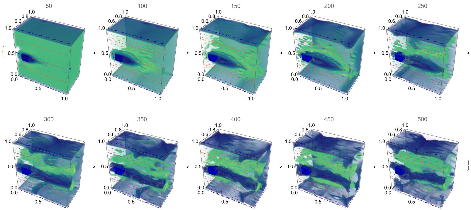
This algorithm is 3D extension of our 2D algorithm published on this page and here. We suppose that with this code we can simulate transition from laminar to turbulent flow. In this example we compute viscous flow around cuboid at Reynolds number $Re=6250$. Note, that code has been tested up to $Re=10^6$.
dif = 1/6250; pec = .72; U0 = 1.; V0 = 0.; W0 = 0.; dn0 = 1.; n = 80;
n1 = n + 1; sm = 500; r = 20; den = ConstantArray[dn0 , {n1, n1, n1}];
u0 = ConstantArray[U0, {n1, n1, n1}];
v0 = ConstantArray[V0, {n1, n1, n1}]; w0 =
 ConstantArray[W0, {n1, n1, n1}]; Do[u0[[i, j, k]] = 0;
 v0[[i, j, k]] = 0;
 w0[[i, j, k]] = 0;, {i, 10, 20, 1}, {j, Round[n/2 - 5],
  Round[n/2 + 5], 1}, {k, Round[n/2 - 5], Round[n/2 + 5], 1}];

periodic[n_, up_, ud_, ul_, ur_, ub_] :=
  Module[{bd = ub},
   Do[bd[[n + 1, i, j]] = bd[[2, i, j]];
    bd[[1, i, j]] = bd[[n, i, j]];, {i, 2, n}, {j, 2, n}];
   Do[bd[[i, 1, j]] = ud;
    bd[[i, n + 1, j]] = up; bd[[i, j, 1]] = ul;
    bd[[i, j, n + 1]] = ur;, {i, 1, n + 1}, {j, 1, n + 1}];
   bd];

diffuse[n_, r_, a_, c_, c0_] :=
  Module[{c1 = c},
   Do[Do[Do[
       Do[c1[[i, j,
            k]] = (c0[[i, j, k]] +
              a (c1[[i - 1, j, k]] + c1[[i + 1, j, k]] +
                 c1[[i, j - 1, k]] + c1[[i, j + 1, k]] +
                 c1[[i, j, k - 1]] + c1[[i, j, k + 1]]))/(1 +
              6 a);, {k, 2, n}];, {j, 2, n}];, {i, 2, n}];
    Do[c1[[i, j, k]] = 0;, {i, 10, 20, 1}, {j, Round[n/2 - 5],
      Round[n/2 + 5], 1}, {k, Round[n/2 - 5], Round[n/2 + 5],
      1}];, {k1, 0, r}];
   c1];

advect[n_, d0_, u_, v_, w_, dt_] :=
  Module[{x, y, z, d1, dt0, i0, i1, j0, j1, k0, k1, s0, s1, t0, t1,
    p1, p0, d000, d100, d010, d001, d110, d011, d101, d111},
   d1 = ConstantArray[0, {n + 1, n + 1, n + 1}]; dt0 = dt n;
   Do[Do[Do[x = i - dt0 u[[i, j, k]]; y = j - dt0 v[[i, j, k]];
        z = k - dt0 w[[i, j, k]];
        i0 = Which[x <= 1, 1, 1 < x < n, Floor[x], True, n];
        i1 = i0 + 1;
        j0 = Which[y <= 1, 1, 1 < y < n, Floor[y], True, n];
        j1 = j0 + 1;
        k0 = Which[z <= 1, 1, 1 < z < n, Floor[z], True, n];
        k1 = k0 + 1;
        d000 = (d0[[i0, j0,
            k0]] + (x - i0) (d0[[i1, j0, k0]] -
              d0[[i0, j0, k0]]) + (y - j0) (d0[[i0, j1, k0]] -
              d0[[i0, j0, k0]]) + (z - k0) (d0[[i0, j0, k1]] -
              d0[[i0, j0, k0]]));
        d100 = (d0[[i1, j0,
            k0]] + (x - i1) (d0[[i1, j0, k0]] -
              d0[[i0, j0, k0]]) + (y - j0) (d0[[i1, j1, k0]] -
              d0[[i1, j0, k0]]) + (z - k0) (d0[[i1, j0, k1]] -
              d0[[i1, j0, k0]]));
        d010 = (d0[[i0, j1,
            k0]] + (x - i0) (d0[[i1, j1, k0]] -
              d0[[i0, j1, k0]]) + (y - j1) (d0[[i0, j1, k0]] -
              d0[[i0, j0, k0]]) + (z - k0) (d0[[i0, j1, k1]] -
              d0[[i0, j1, k0]]));
        d001 = (d0[[i0, j0,
            k1]] + (x - i0) (d0[[i1, j0, k1]] -
              d0[[i0, j0, k1]]) + (y - j0) (d0[[i0, j1, k1]] -
              d0[[i0, j0, k1]]) + (z - k1) (d0[[i0, j0, k1]] -
              d0[[i0, j0, k0]]));
        d110 = (d0[[i1, j1,
            k0]] + (x - i1) (d0[[i1, j1, k0]] -
              d0[[i0, j1, k0]]) + (y - j1) (d0[[i1, j1, k0]] -
              d0[[i1, j0, k0]]) + (z - k0) (d0[[i1, j1, k1]] -
              d0[[i1, j1, k0]]));
        d011 = (d0[[i0, j1,
            k1]] + (x - i0) (d0[[i1, j1, k1]] -
              d0[[i0, j1, k1]]) + (y - j1) (d0[[i0, j1, k1]] -
              d0[[i0, j0, k1]]) + (z - k1) (d0[[i0, j1, k1]] -
              d0[[i0, j1, k0]]));
        d101 = (d0[[i1, j0,
            k1]] + (x - i1) (d0[[i1, j0, k1]] -
              d0[[i0, j0, k1]]) + (y - j0) (d0[[i1, j1, k1]] -
              d0[[i1, j0, k1]]) + (z - k1) (d0[[i1, j0, k1]] -
              d0[[i1, j0, k0]]));
        d111 = (d0[[i1, j1,
            k1]] + (x - i1) (d0[[i1, j1, k1]] -
              d0[[i0, j1, k1]]) + (y - j1) (d0[[i1, j1, k1]] -
              d0[[i1, j0, k1]]) + (z - k1) (d0[[i1, j1, k1]] -
              d0[[i1, j1, k0]]));
        d1[[i, j,
          k]] = (d000 + d100 + d010 + d001 + d110 + d011 + d101 +
            d111)/8;, {k, 2, n}];, {j, 2, n}];, {i, 1, n + 1}]; d1];

project[n_, r_, u0_, v0_, w0_, u_, v_, w_] :=
  Module[{ux = u, vy = v, wz = w, div, p},
   p = ConstantArray[0, {n + 1, n + 1, n + 1}];
   div = ConstantArray[0, {n + 1, n + 1, n + 1}];
   ux = ConstantArray[0, {n + 1, n + 1, n + 1}];
   vy = ConstantArray[0, {n + 1, n + 1, n + 1}];
   wz = ConstantArray[0, {n + 1, n + 1, n + 1}];
   Do[div[[i, j,
       k]] = .5/
        n (u0[[i + 1, j, k]] - u0[[i - 1, j, k]] + v0[[i, 1 + j, k]] -
          v0[[i, j - 1, k]] + w0[[i, j, k + 1]] -
         w0[[i, j, k - 1]]);, {i, 2, n}, {j, 2, n}, {k, 2, n}];
   Do[div[[i, j, k]] = 0;, {i, 10, 20, 1}, {j, Round[n/2 - 5],
     Round[n/2 + 5], 1}, {k, Round[n/2 - 5], Round[n/2 + 5], 1}];
   div = periodic[n, 0, 0, 0, 0, div];
   Do[Do[Do[
       Do[p[[i, j,
            k]] = (div[[i, j,
               k]] + (p[[i - 1, j, k]] + p[[i + 1, j, k]] +
                p[[i, j - 1, k]] + p[[i, j + 1, k]] +
                p[[i, j, k - 1]] + p[[i, j, k + 1]]))/6;, {k, 2,
          n}];, {j, 2, n}], {i, 2, n}];, {k1, 0, r}];
   Do[p[[i, j, k]] = 0;, {i, 10, 20, 1}, {j, Round[n/2 - 5],
     Round[n/2 + 5], 1}, {k, Round[n/2 - 5], Round[n/2 + 5], 1}];
   p = periodic[n, 0, 0, 0, 0, p];
   Do[ux[[i, j, k]] =
     u0[[i, j, k]] + .5 n (p[[i + 1, j, k]] - p[[i - 1, j, k]]);
    vy[[i, j, k]] =
     v0[[i, j, k]] + .5 n (p[[i, j + 1, k]] - p[[i, j - 1, k]]);
    wz[[i, j, k]] =
     w0[[i, j, k]] + .5 n (p[[i, j, k + 1]] - p[[i, j, k - 1]]);, {i,
     2, n}, {j, 2, n}, {k, 2, n}];
   Do[ux[[i, j, k]] = 0; vy[[i, j, k]] = 0;
    wz[[i, j, k]] = 0;, {i, 10, 20, 1}, {j, Round[n/2 - 5],
     Round[n/2 + 5], 1}, {k, Round[n/2 - 5], Round[n/2 + 5], 1}]; {ux,
     vy, wz}];

onestep[n_, step_, r_, a_, uin_, vin_, win_, dt_, c_] :=
 Module[{u1, v1, w1, u, v, w, u0, v0, w0},
  u0 = ConstantArray[0., {n + 1, n + 1, n + 1}];
  v0 = ConstantArray[0., {n + 1, n + 1, n + 1}];
  w0 = ConstantArray[0., {n + 1, n + 1, n + 1}];
  u = ConstantArray[0., {n + 1, n + 1, n + 1}];
  v = ConstantArray[0., {n + 1, n + 1, n + 1}];
  w = ConstantArray[0., {n + 1, n + 1, n + 1}];
  u1 = ConstantArray[0., {n + 1, n + 1, n + 1}];
  v1 = ConstantArray[0., {n + 1, n + 1, n + 1}];
  w1 = ConstantArray[0., {n + 1, n + 1, n + 1}]; u0 = uin; v0 = vin;
  w0 = win;
  Do[u0[[i, j, k]] = 0; v0[[i, j, k]] = 0;
   w0[[i, j, k]] = 0;, {i, 10, 20, 1}, {j, Round[n/2 - 5],
    Round[n/2 + 5], 1}, {k, Round[n/2 - 5], Round[n/2 + 5], 1}];
  u0 = advect[n, u0, u0, v0, w0, dt];
  v0 = advect[n, v0, u0, v0, w0, dt];
  w0 = advect[n, w0, u0, v0, w0, dt];
  Do[u0[[i, j, k]] = 0;
   v0[[i, j, k]] = 0;, {i, 10, 20, 1}, {j, Round[n/2 - 5],
    Round[n/2 + 5], 1}, {k, Round[n/2 - 5], Round[n/2 + 5], 1}];
  u0 = periodic[n, 0, 0, 0, 0, u0]; v0 = periodic[n, 0, 0, 0, 0, v0];
  w0 = periodic[n, 0, 0, 0, 0, w0];
  u0 = diffuse[n, r, a, c, u0]; v0 = diffuse[n, r, a, c, v0];
  w0 = diffuse[n, r, a, c, w0];
  Do[u0[[i, j, k]] = 0; v0[[i, j, k]] = 0;
   w0[[i, j, k]] = 0;, {i, 10, 20, 1}, {j, Round[n/2 - 5],
    Round[n/2 + 5], 1}, {k, Round[n/2 - 5], Round[n/2 + 5], 1}];
  u0 = periodic[n, 0, 0, 0, 0, u0]; v0 = periodic[n, 0, 0, 0, 0, v0];
  w0 = periodic[n, 0, 0, 0, 0, w0];
  {u0, v0, w0} = project[n, r, u0, v0, w0, u, v, w];
  Do[u0[[i, j, k]] = 0; v0[[i, j, k]] = 0;
   w0[[i, j, k]] = 0;, {i, 10, 20, 1}, {j, Round[n/2 - 5],
    Round[n/2 + 5], 1}, {k, Round[n/2 - 5], Round[n/2 + 5], 1}];
  u0 = periodic[n, 0, 0, 0, 0, u0]; v0 = periodic[n, 0, 0, 0, 0, v0];
  w0 = periodic[n, 0, 0, 0, 0, w0]; {u0, v0, w0}]

cf = With[{cg = Compile`GetElement, hp = HoldPattern,
     dv = DownValues},
    Hold@Compile[{{u0argu, _Real, 3}, {v0argu, _Real,
              3}, {w0argu, _Real, 3}, {denargu, _Real,
              3}, {sm, _Integer}, {n, _Integer}, {r, _Integer}, dif,
             pec}, Module[{u0 = u0argu, v0 = v0argu, w0 = w0argu, uu,
              vv, ww, dd, den = denargu,
              c = Table[0., {n + 1}, {n + 1}, {n + 1}], dt = 40./n^2,
              a, dnup = den[[1, n + 1, 1]], dnd = den[[1, 1, 1]],
              dnl = den[[1, 1, 1]], dnr = den[[1, 1, n + 1]]},
             a = dt dif n n;

             uu = vv =
               ww = dd =
                 Table[0., {sm + 1}, {n + 1}, {n + 1}, {n + 1}];

             Do[{u0, v0, w0} =
               onestep[n, step, r, a, u0, v0, w0, dt, c];
              uu[[step + 1]] = u0;
              vv[[step + 1]] = v0; ww[[step + 1]] = w0;
              den = diffuse[n, r, a/pec, c, den];
              Do[den[[i, j, k]] = 0;, {i, 10, 20, 1}, {j,

                   Round[n/2 - 5], Round[n/2 + 5], 1}, {k,
                Round[n/2 - 5], Round[n/2 + 5], 1}];
              den = periodic[n, dnup, dnd, dnl, dnr, den];
              den = advect[n, den, u0, v0, w0, dt];
              Do[den[[i, j, k]] = 0;, {i, 10, 20, 1}, {j,
                Round[n/2 - 5], Round[n/2 + 5], 1}, {k,
                Round[n/2 - 5], Round[n/2 + 5], 1}];
              den = periodic[n, dnup, dnd, dnl, dnr, den];
              dd[[step + 1]] = den;, {step, 0, sm}]; {uu, vv, ww,
              dd}], CompilationTarget -> "C",
            RuntimeOptions -> "Speed"] /. dv@onestep /.
         Flatten[dv /@ {advect, diffuse, periodic, project}] /.
        hp@ConstantArray[c_, {i_, j_, kc_}] :>
         Table[0., {i}, {j}, {kc}] /. hp@Part[a__] :> cg[a] /.
      hp[cg[a__] = rhs_] :> (Part[a] = rhs) //
     ReleaseHold];


rst = cf[u0, v0, w0, den, sm, n, r, dif, pec];
Visualization
Do[lst11[s] =
  Table[{{(i - 1)/n, (j - 1)/n, (k - 1)/n}, rst[[1, s, i, j, k]]}, {i,
     n1}, {j, n1}, {k, n1}];
 lst12[s] =
  Table[{{(i - 1)/n, (j - 1)/n, (k - 1)/n}, rst[[2, s, i, j, k]]}, {i,
     n1}, {j, n1}, {k, n1}];
 lst13[s] =
  Table[{{(i - 1)/n, (j - 1)/n, (k - 1)/n}, rst[[3, s, i, j, k]]}, {i,
     n1}, {j, n1}, {k, n1}];, {s, 25, sm, 25}]

Do[su1[i] =
  Interpolation[Flatten[lst11[i], 2], InterpolationOrder -> 3];
 sv2[i] = Interpolation[Flatten[lst12[i], 2],
   InterpolationOrder -> 3];
 sw3[i] = Interpolation[Flatten[lst13[i], 2],
   InterpolationOrder -> 3];, {i, 25, sm, 25}]

Table[Show[
  DensityPlot3D[
   Norm[{su1[i][x, y, z], sv2[i][x, y, z], sw3[i][x, y, z]}], {x, 0,
    1}, {y, 0.44, 1}, {z, 0, 1}, BoxRatios -> Automatic,
   ColorFunction -> "BlueGreenYellow", PlotLabel -> i],
  VectorPlot3D[{su1[i][x, y, z], sv2[i][x, y, z],
    sw3[i][x, y, z]}, {x, 0, 1}, {y, 0, .5}, {z, 0, 1},
   VectorPoints -> Fine, VectorMarkers -> "Arrow"],
  Graphics3D[{{Blue,
     Cuboid[{10, Round[n/2 - 5] - 1/2,
        Round[n/2 - 5] - 1/2}/(n + 1), {20, Round[n/2 + 5] - 1/2,
        Round[n/2 + 5] - 1/2}/(n + 1)]}}]], {i, 50, sm, 50}]
Animation
Do[lstu1[k] =
Flatten[Table[{{(i - 1)/n, (j - 1)/n},
rst[[1, k, i, Round[(n + 1)/2], j]]}, {i, n1}, {j, n1}], 1];
lstw1[k] =
Flatten[Table[{{(i - 1)/n, (j - 1)/n},
rst[[2, k, i, Round[(n + 1)/2], j]]}, {i, n1}, {j, n1}],
1];, {k, sm}];
Do[Uvel1[i] = Interpolation[lstu1[i], InterpolationOrder -> 3];, {i,
1, sm}];
Do[Wvel1[i] = Interpolation[lstw1[i], InterpolationOrder -> 3];, {i,
1, sm}];
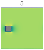
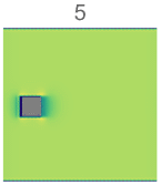
frame = Table[
Show[DensityPlot[
Norm[{Uvel[m][x, y], Vvel[m][x, y]}], {x, 0, 1}, {y, 0, 1},
PlotRange -> All, ColorFunction -> "BlueGreenYellow",
Frame -> False, ImageSize -> Tiny, PlotLabel -> m,
PlotPoints -> 50],
Graphics[{Gray,
Rectangle[{10, Round[n/2 - 5] - 1/2}/(n + 1), {20,
Round[n/2 + 5] - 1/2}/(n + 1)]}]], {m, 5, sm, 3}];
The question is about code improvement. How can we define parameter r to solve Laplace and Poison equations in this code? Note, r is number of iterations in diffuse and project module (we use Gauss-Seidel relaxation to solve Laplace and Poison's equations).
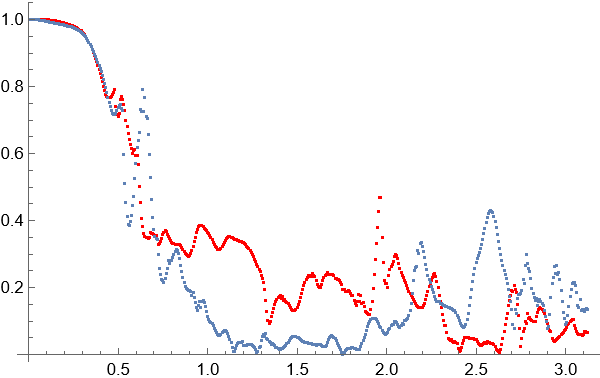
Update 1. We can reduce r from r=20 as above to r=5 as below. Globally there is no difference in two animations.
But if we compare velocity in some point like $x=0.65, y=0.5$ then we have good agreement for $r=5$ (red points) and $r=20$ (gray points) in laminar flow at $t<0.5$, but a big difference in the turbulent flow at $t>0.5$.
Update 1. To test the Gauss-Seidel relaxation method itself we can compute viscous flow in a plane channel with external force (gravity) as follows
ClearAll["Global`*"]

dif = 1/80; pec = 1; U0 = 0; V0 = 0; n = 11; n1 = n + 1; dt =
 2./n^2; sm = 3000; r = 7; n2 = Round[n/2]; a = dt dif n n; c =
 ConstantArray[0, {n1, n1}]; c0 = ConstantArray[0, {n1, n1}];; u0 =
 ConstantArray[0, {n1, n1}]; v0 = ConstantArray[0, {n1, n1}]; u =
 ConstantArray[0, {n1, n1}]; v = ConstantArray[0, {n1, n1}];

periodic[n_, up_, ud_, ub_] :=
  Module[{bd = ub},
   Do[bd[[1, i]] = .5 (bd[[n, i]] + bd[[2, i]]);
    bd[[n + 1, i]] = bd[[1, i]]; bd[[i, 1]] = ud;
    bd[[i, n + 1]] = up;, {i, 2, n}]; bd[[1, 1]] = ud;
   bd[[n + 1, n + 1]] = up; bd[[n + 1, 1]] = ud; bd[[1, n + 1]] = up;
   bd];

diffuse[n_, r_, a_, c_, c0_] :=
 Module[{c1 = c}, c1 = ConstantArray[0, {n + 1, n + 1}];
  Do[Do[Do[c1[[i,
         j]] = (c0[[i, j]] +
           a (c1[[i - 1, j]] + c1[[i + 1, j]] + c1[[i, j - 1]] +
              c1[[i, j + 1]]))/(1 + 4 a);, {j, 2, n}];, {i, 2, n}];
   c1 = periodic[n, 0, 0, c1];, {k, 0, r}]; c1];
advect[n_, b_, d_, d0_, u_, v_, dt_] :=
 Module[{x, y}, d1 = ConstantArray[0, {n + 1, n + 1}]; dt0 = dt n;
  Do[Do[x = i - dt0 u[[i, j]]; y = j - dt0 v[[i, j]];
     i0 = Which[x <= 1, 1, 1 < x < n, Floor[x], x >= n, n];
     i1 = i0 + 1;
     j0 = Which[y <= 1, 1, 1 < y < n, Floor[y], y >= n, n];
     j1 = j0 + 1; s1 = x - i0; s0 = 1 - s1; t1 = y - j0; t0 = 1 - t1;
     d1[[i, j]] =
      s0 (t0 d0[[i0, j0]] + t1 d0[[i0, j1]]) +
       s1 (t0 d0[[i1, j0]] + t1 d0[[i1, j1]]);, {j, 1, n + 1}];, {i,
    1, n + 1}]; d1];
project[n_, r_, u0_, v0_, u_, v_] :=
  Module[{ux = u, vy = v}, p = ConstantArray[0, {n1, n1}];
   div = ConstantArray[0, {n1, n1}]; ux = ConstantArray[0, {n1, n1}];
   vy = ConstantArray[0, {n1, n1}];
   Do[div[[i,
       j]] = -.5 /
        n (u0[[i + 1, j]] - u0[[i - 1, j]] + v0[[i, 1 + j]] -
         v0[[i, j - 1]]);, {i, 2, n}, {j, 2, n}];
   Do[Do[Do[
       p[[i, j]] = (div[[i,
             j]] + (p[[i - 1, j]] + p[[i + 1, j]] + p[[i, j - 1]] +
              p[[i, j + 1]]))/4;, {j, 2, n}], {i, 2, n}];, {k, 0, r}];
    Do[ux[[i, j]] = u0[[i, j]] - .5 n (p[[i + 1, j]] - p[[i - 1, j]]);
     vy[[i, j]] =
     v0[[i, j]] - .5 n (p[[i, j + 1]] - p[[i, j - 1]]);, {i, 2,
     n}, {j, 2, n}]; {ux, vy}];
(*force*)
Fx[t_, x_, y_] := 1/10; Fy[t_, x_, y_] := 0;
f1 = ConstantArray[0, {n1, n1}]; f2 = ConstantArray[0, {n1, n1}];

Do[u0 = advect[n, 0, c, u0, u0, v0, dt];
  v0 = advect[n, 0, c, v0, u0, v0, dt];
  u0 = periodic[n, 0, 0, u0]; v0 = periodic[n, 0, 0, v0];
  u0 = diffuse[n, r, a, c, u0]; v0 = diffuse[n, r, a, c, v0];
  u0 = periodic[n, 0, 0, u0]; v0 = periodic[n, 0, 0, v0];
  Do[f1[[i, j]] = Fx[dt (step + .5), (i - 1)/n, (j - 1)/n];
   f2[[i, j]] = Fy[dt (step + .5), (i - 1)/n, (j - 1)/n];, {i, 2,
    n1}, {j, 2, n1}]; u0 += f1 dt;
  v0 += f2 dt; {u0, v0} = project[n, r, u0, v0, u, v];
  u0 = periodic[n, 0, 0, u0]; v0 = periodic[n, 0, 0, v0];
  uu[step] = u0; vv[step] = v0;, {step, 0, sm}];
Visualization of flow velocity and absolute error
Do[lstu[k] =
   Flatten[Table[{{(i - 1)/n, (j - 1)/n}, uu[k][[i, j]]}, {i, n1}, {j,
       n1}], 1];
  lstv[k] =
   Flatten[Table[{{(i - 1)/n, (j - 1)/n}, vv[k][[i, j]]}, {i, n1}, {j,
       n1}], 1];, {k, 0, sm}];
Do[Uvel[i] = Interpolation[lstu[i], InterpolationOrder -> 3];, {i, 1,
  sm}]
Do[Vvel[i] = Interpolation[lstv[i], InterpolationOrder -> 3];, {i, 1,
   sm}];

{StreamDensityPlot[{Uvel[sm][x, y], Vvel[sm][x, y]}, {x, 0, 1}, {y, 0,
    1}, ColorFunction -> "RoseColors", Frame -> False,
  PlotLegends -> Automatic],
 Plot3D[Uvel[sm][x, y], {x, 0, 1}, {y, 0, 1},
  ColorFunction -> "RoseColors"]}

{ListPlot[Table[{i dt, Max[uu[i]]}, {i, sm}],
  AxesLabel -> {"t", "Umax"}],
 Plot[{-4 (-y + y^2), Uvel[sm][.5, y]}, {y, 0, 1},
  PlotStyle -> {Thick, {Red, Dashed}}, Frame -> True,
  FrameLabel -> {"y", "u"},
  PlotLegends -> {"Exact solution", "Numeric solution"}],
 Plot[Abs[-Uvel[sm][.5, y] - 4 (-y + y^2)], {y, 0, 1}, Frame -> True,
  FrameLabel -> {"y", "Error"}]}
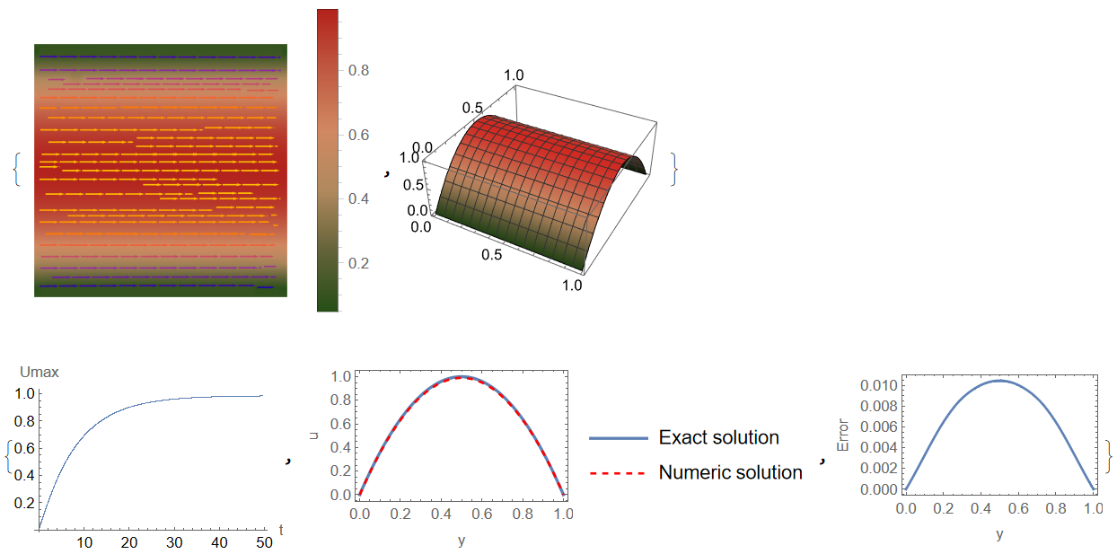
Actually for r=7 we have a good convergence to the exact solution on the grid of 12 points with error of $10^{−2}$. For r=5 the error is about 0.2 and for r=10 error is about $10^{−2}$, therefore r=7 is optimal value.
Update 2. In the module advect we can use trilinear interpolation as follows
advect[n_, d0_, u_, v_, w_, dt_] :=
  Module[{x, y, z, d1, dt0, i0, i1, j0, j1, k0, k1, s0, s1, t0, t1,
    p1, p0, d00, d10, d01, d11, cd0, cd1, xd, yd, zd},
   d1 = ConstantArray[0, {n + 1, n + 1, n + 1}]; dt0 = dt n;
   Do[Do[Do[x = i - dt0 u[[i, j, k]]; y = j - dt0 v[[i, j, k]];
        z = k - dt0 w[[i, j, k]];
        i0 = Which[x <= 1, 1, 1 < x < n, Floor[x], True, n];
        i1 = i0 + 1;
        j0 = Which[y <= 1, 1, 1 < y < n, Floor[y], True, n];
        j1 = j0 + 1;
        k0 = Which[z <= 1, 1, 1 < z < n, Floor[z], True, n];
        k1 = k0 + 1;(*Trilinear interpolation*)xd = x - i0;
        yd = y - j0; zd = z - k0;
        d00 = d0[[i0, j0, k0]] (1 - xd) + d0[[i1, j0, k0]] xd;
        d01 = d0[[i0, j0, k1]] (1 - xd) + d0[[i1, j0, k1]] xd;
        d10 = d0[[i0, j1, k0]] (1 - xd) + d0[[i1, j1, k0]] xd;
        d11 = d0[[i0, j1, k1]] (1 - xd) + d0[[i1, j1, k1]] xd;
        cd0 = d00 (1 - yd) + d10 yd; cd1 = d01 (1 - yd) + d11 yd;
        d1[[i, j, k]] = cd0 (1 - zd) + cd1 zd;
        , {k, 2, n}];, {j, 2, n}];, {i, 1, n + 1}]; d1];
Update: testing projection step
To test projection step itself we can use Mathematica FEM and exact benchmark solution from well known paper EXACT FULLY 3D NAVIER-STOKES SOLUTIONS FOR BENCHMARKING by C. ROSS ETHIER AND D. A. STEINMAN as follows. First, we consider projection step as an implementation of the predictor-corrector algorithm $$\frac{u-u_n}{\tau}+(u.\nabla)u-\nu\nabla^2 u=0$$ $$\frac{u_{n+1}-u}{\tau}+\nabla p =0$$ here $\tau$ is time step, $u_n, u, u_{n+1}$ if velocity field on previous, intermediate and next step consequently, and $p$ is a pressure. We suppose that $\nabla.u_{n+1}=0$, and therefore $$\nabla^2p-\frac{\nabla.u}{\tau}=0$$ Second, we solve NSE in the unit cuboid with Dirichlet condition using exact solution and FEM, we have code
Clear["Global`*"]
Needs["NDSolve`FEM`"]
reg = Cuboid[];
mesh = ToElementMesh[reg, MaxCellMeasure -> 0.001];
(*Exact solution*)
U[x_, y_, z_,
  t_] := -a Exp[-d^2 t] (Exp[a x] Sin[a y + d z] +
    Exp[a z] Cos[a x + d y]);
V[x_, y_, z_,
  t_] := -a Exp[-d^2 t] (Exp[a y] Sin[a z + d x] +
    Exp[a x] Cos[a y + d z]);
W[x_, y_, z_,
  t_] := -a Exp[-d^2 t] (Exp[a z] Sin[a x + d y] +
    Exp[a y] Cos[a z + d x]);
P[x_, y_, z_,
  t_] := -a ^2/
   2 Exp[-2 d^2 t] (Exp[2 a x] + Exp[2 a y] + Exp[2 a z] +
    2 Sin[a x + d y] Exp[a (y + z)] Cos[a z + d x] +
    2 Sin[a y + d z] Exp[a (x + z)] Cos[a x + d y] +
    2 Sin[a z + d x] Exp[a (y + x)] Cos[
      a y + d z]);
(*t0 is time step, nn is number of iterations *)
a = 1; d = 1; t0 = 1/400; nn = 200; \[Nu] = 1;
(*FEM implementation of predictor-corrector algorithm*)
UX[0] = U[x, y, z, 0];
VY[0] = V[x, y, z, 0]; WZ[0] = W[x, y, z, 0];
P0[0] = P[x, y, z, 0];
Do[
   {UX[i], VY[i], WZ[i], P0[i]} =
     NDSolveValue[{{-\[Nu]*
           Laplacian[
            u[x, y, z], {x, y, z}] + (u[x, y, z] - UX[i - 1])/t0 +
          UX[i - 1]*D[u[x, y, z], x] + VY[i - 1]*D[u[x, y, z], y] +
          WZ[i - 1]*D[u[x, y, z], z], -\[Nu]*
           Laplacian[
            v[x, y, z], {x, y, z}] + (v[x, y, z] - VY[i - 1])/t0 +
          UX[i - 1]*D[v[x, y, z], x] + VY[i - 1]*D[v[x, y, z], y] +
          WZ[i - 1]*D[v[x, y, z], z], -\[Nu]*
           Laplacian[
            w[x, y, z], {x, y, z}] + (w[x, y, z] - WZ[i - 1])/t0 +
          UX[i - 1]*D[w[x, y, z], x] + VY[i - 1]*D[w[x, y, z], y] +
          WZ[i - 1]*D[w[x, y, z], z],
         Laplacian[p[x, y, z], {x, y, z}] - (
\!\(\*SuperscriptBox[\(u\),
TagBox[
RowBox[{"(",
RowBox[{"1", ",", "0", ",", "0"}], ")"}],
Derivative],
MultilineFunction->None]\)[x, y, z] +
\!\(\*SuperscriptBox[\(v\),
TagBox[
RowBox[{"(",
RowBox[{"0", ",", "1", ",", "0"}], ")"}],
Derivative],
MultilineFunction->None]\)[x, y, z] +
\!\(\*SuperscriptBox[\(w\),
TagBox[
RowBox[{"(",
RowBox[{"0", ",", "0", ",", "1"}], ")"}],
Derivative],
MultilineFunction->None]\)[x, y, z])/t0} == {0, 0, 0, 0}, {
        DirichletCondition[{u[x, y, z] ==
           U[x, y, z, i t0 - t0/2] + t0 D[P[x, y, z, i t0], x],
          v[x, y, z] ==
           V[x, y, z, i t0 - t0/2] + t0 D[P[x, y, z, i t0], y],
          w[x, y, z] ==
           W[x, y, z, i t0 - t0/2] + t0 D[P[x, y, z, i t0], z],
          p[x, y, z] == P[x, y, z, i t0 ]}, True]}}, {u[x, y, z] - t0
\!\(\*SuperscriptBox[\(p\),
TagBox[
RowBox[{"(",
RowBox[{"1", ",", "0", ",", "0"}], ")"}],
Derivative],
MultilineFunction->None]\)[x, y, z], v[x, y, z] - t0
\!\(\*SuperscriptBox[\(p\),
TagBox[
RowBox[{"(",
RowBox[{"0", ",", "1", ",", "0"}], ")"}],
Derivative],
MultilineFunction->None]\)[x, y, z], w[x, y, z] - t0
\!\(\*SuperscriptBox[\(p\),
TagBox[
RowBox[{"(",
RowBox[{"0", ",", "0", ",", "1"}], ")"}],
Derivative],
MultilineFunction->None]\)[x, y, z],
       p[x, y, z]}, {x, y, z} \[Element] mesh,
      Method -> {"FiniteElement",
        "InterpolationOrder" -> {u -> 2, v -> 2, w -> 2,
          p -> 2}}];, {i, 1, nn}];
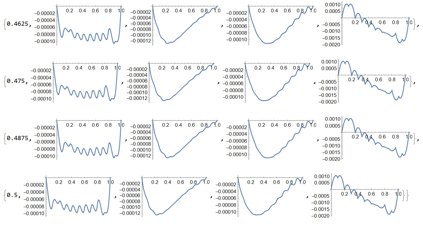
Visualization of error on every 5 steps on the line $x=1/2, z=1/2$ for $u_n=(UX[n],VY[n],WZ[n])$, and $p=P0[n]$
Table[{k t0 // N,
  Plot[Evaluate[{U[x, y, z, k t0]/UX[k] - 1} /. {x -> 1/2,
      z -> 1/2}], {y, 0, 1}, PlotRange -> All],
  Plot[Evaluate[{V[x, y, z, k t0]/VY[k] - 1} /. {x -> 1/2,
      z -> 1/2}], {y, 0, 1}, PlotRange -> All],
  Plot[Evaluate[{W[x, y, z, k t0]/WZ[k] - 1} /. {x -> 1/2,
      z -> 1/2}], {y, 0, 1}, PlotRange -> All],
  Plot[Evaluate[{P[x, y, z, k t0]/P0[k] - 1} /. {x -> 1/2,
      z -> 1/2}], {y, 0, 1}, PlotRange -> All]}, {k, 5, nn, 5}]
Please note, that in the picture shown last steps only. The relative error for pressure is about $3\times 10^{-3}$, and for velocity $1.25\times10^{-3}$ on the grid $10\times10\times 10$ on 200 steps in time with time step $\tau =1/400$. 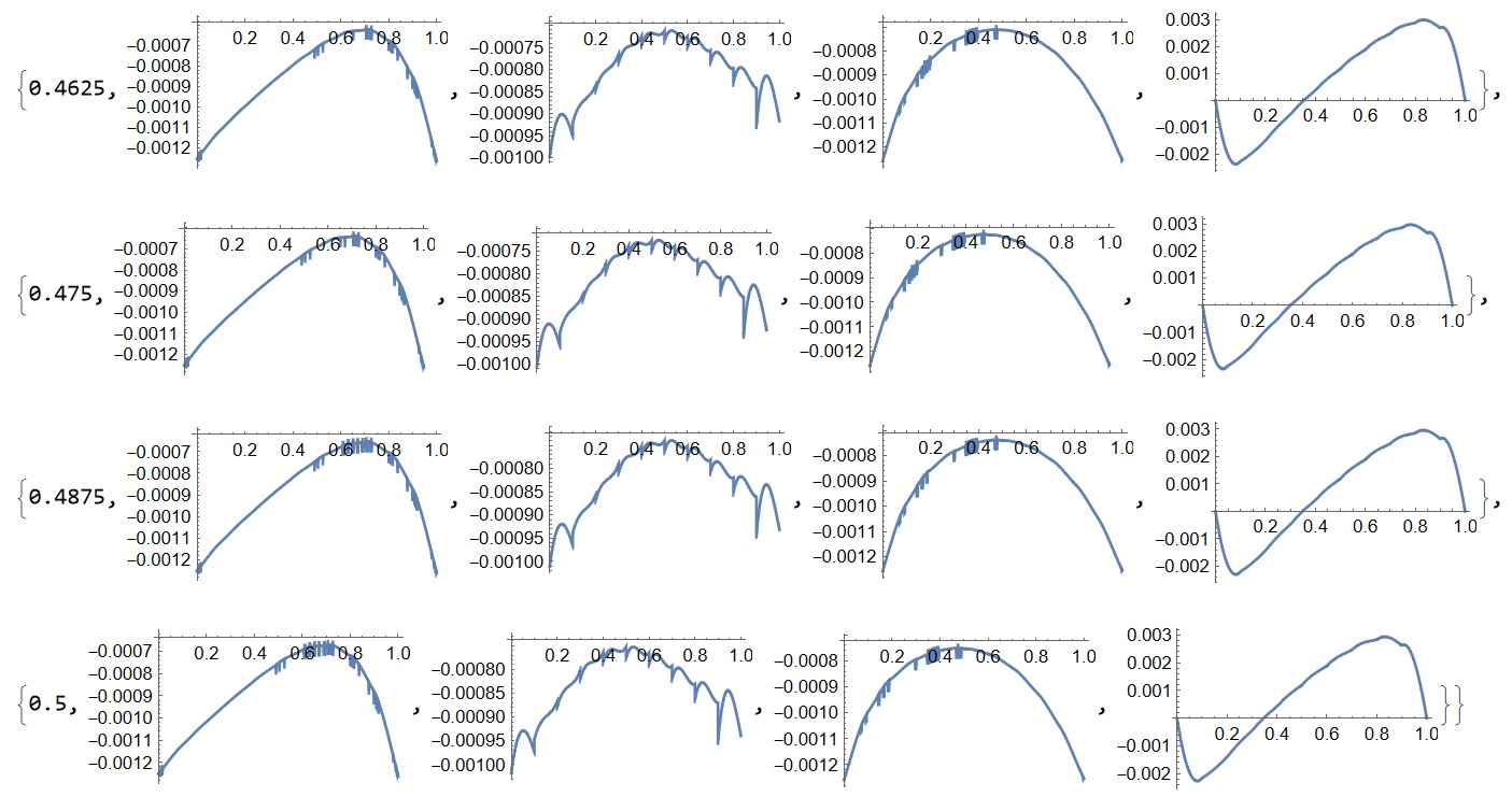
Using exact benchmark solution we also can test linear FEM algorithm described on Solver for unsteady flow with the use of Mathematica FEM and extended to 3D below as follows
Needs["NDSolve`FEM`"]
reg = Cuboid[];
mesh = ToElementMesh[reg, MaxCellMeasure -> 0.001]

U[x_, y_, z_,
  t_] := -a Exp[-d^2 t] (Exp[a x] Sin[a y + d z] +
    Exp[a z] Cos[a x + d y]);
V[x_, y_, z_,
  t_] := -a Exp[-d^2 t] (Exp[a y] Sin[a z + d x] +
    Exp[a x] Cos[a y + d z]);
W[x_, y_, z_,
  t_] := -a Exp[-d^2 t] (Exp[a z] Sin[a x + d y] +
    Exp[a y] Cos[a z + d x]);
P[x_, y_, z_,
  t_] := -a ^2/
   2 Exp[-2 d^2 t] (Exp[2 a x] + Exp[2 a y] + Exp[2 a z] +
    2 Sin[a x + d y] Exp[a (y + z)] Cos[a z + d x] +
    2 Sin[a y + d z] Exp[a (x + z)] Cos[a x + d y] +
    2 Sin[a z + d x] Exp[a (y + x)] Cos[
      a y + d z]); a = 1; d = 1; t0 = 1/400; nn = 200; \[Nu] = 1;
UX[0] = U[x, y, z, 0];
VY[0] = V[x, y, z, 0]; WZ[0] = W[x, y, z, 0];
P0[0] = P[x, y, z, 0];
Do[
   {UX[i], VY[i], WZ[i], P0[i]} =
     NDSolveValue[{{-\[Nu]*
           Laplacian[
            u[x, y, z], {x, y, z}] + (u[x, y, z] - UX[i - 1])/t0 +
          UX[i - 1]*D[u[x, y, z], x] + VY[i - 1]*D[u[x, y, z], y] +
          WZ[i - 1]*D[u[x, y, z], z] +
\!\(\*SuperscriptBox[\(p\),
TagBox[
RowBox[{"(",
RowBox[{"1", ",", "0", ",", "0"}], ")"}],
Derivative],
MultilineFunction->None]\)[x, y, z], -\[Nu]*
           Laplacian[
            v[x, y, z], {x, y, z}] + (v[x, y, z] - VY[i - 1])/t0 +
          UX[i - 1]*D[v[x, y, z], x] + VY[i - 1]*D[v[x, y, z], y] +
          WZ[i - 1]*D[v[x, y, z], z] +
\!\(\*SuperscriptBox[\(p\),
TagBox[
RowBox[{"(",
RowBox[{"0", ",", "1", ",", "0"}], ")"}],
Derivative],
MultilineFunction->None]\)[x, y, z], -\[Nu]*
           Laplacian[
            w[x, y, z], {x, y, z}] + (w[x, y, z] - WZ[i - 1])/t0 +
          UX[i - 1]*D[w[x, y, z], x] + VY[i - 1]*D[w[x, y, z], y] +
          WZ[i - 1]*D[w[x, y, z], z] +
\!\(\*SuperscriptBox[\(p\),
TagBox[
RowBox[{"(",
RowBox[{"0", ",", "0", ",", "1"}], ")"}],
Derivative],
MultilineFunction->None]\)[x, y, z], (
\!\(\*SuperscriptBox[\(u\),
TagBox[
RowBox[{"(",
RowBox[{"1", ",", "0", ",", "0"}], ")"}],
Derivative],
MultilineFunction->None]\)[x, y, z] +
\!\(\*SuperscriptBox[\(v\),
TagBox[
RowBox[{"(",
RowBox[{"0", ",", "1", ",", "0"}], ")"}],
Derivative],
MultilineFunction->None]\)[x, y, z] +
\!\(\*SuperscriptBox[\(w\),
TagBox[
RowBox[{"(",
RowBox[{"0", ",", "0", ",", "1"}], ")"}],
Derivative],
MultilineFunction->None]\)[x, y, z])} == {0, 0, 0, 0}, {
        DirichletCondition[{u[x, y, z] == U[x, y, z, i t0],
          v[x, y, z] == V[x, y, z, i t0],
          w[x, y, z] == W[x, y, z, i t0],
          p[x, y, z] == P[x, y, z, i t0]}, True]}}, {u[x, y, z] ,
       v[x, y, z] , w[x, y, z] , p[x, y, z]}, {x, y, z} \[Element]
       mesh, Method -> {"FiniteElement",
        "InterpolationOrder" -> {u -> 2, v -> 2, w -> 2,
          p -> 1}}];, {i, 1, nn}];
Visualization of error on every 5 steps on the line $y=1/2,z=1/2$ for $u_n=(UX[n],VY[n],WZ[n])$, and $p=P0[n]$
Table[{k t0 // N,
  Plot[Evaluate[{U[x, y, z, k t0]/UX[k] - 1} /. {y -> 1/2,
      z -> 1/2}], {x, 0, 1}, PlotRange -> All],
  Plot[Evaluate[{V[x, y, z, k t0]/VY[k] - 1} /. {y -> 1/2,
      z -> 1/2}], {x, 0, 1}, PlotRange -> All],
  Plot[Evaluate[{W[x, y, z, k t0]/WZ[k] - 1} /. {y -> 1/2,
      z -> 1/2}], {x, 0, 1}, PlotRange -> All],
  Plot[Evaluate[{P[x, y, z, k t0]/P0[k] - 1} /. {y -> 1/2,
      z -> 1/2}], {x, 0, 1}, PlotRange -> All]}, {k, 5, nn, 5}]
Note, that in the picture shown last steps only. The relative error for pressure is about $2×10^{−3}$, and for velocity $1.5×10^{−4}$ on the grid 10×10×10 on 200 steps in time with time step τ=1/400.