Message Boards Message Boards

1
|
19461 Views
|
10 Replies
|
6 Total Likes
View groups...
Share
Share this post:

Visualization of Gaussian Curvature

Posted 10 years ago
Hi,
I need to visualize Gaussian Curvature of a parametric surface. there is a solution here:

How to visualize the Gaussian curvature of a 3D surface?

but Im not sure its working because when I draw a sphere its all white but it should be red or brown(because its Gaussian curvature is positive).
how can I modify that code such that for any point on the surface if its Gaussian curvature is positive it turns red and if its zero it turns to white and for negative it turns to blue.
if I can do this with any other software please tell me.
please help me out,(sorry for my bad English).
POSTED BY: Ali Noroozi
10 Replies

Absolutely.

twist = gccolor[{Cos[u] Cos[v], Sin[u] Cos[v], u + Sin[v]}, {u, 0, 2 Pi}, {v, -Pi, Pi}];
Animate[
 With[{v = RotationTransform[\[Theta], {0, 0, 1}][{3, 0, 3}]},
  Show[twist, ViewPoint -> v, SphericalRegion -> True, Boxed -> False, Axes -> False]],
 {\[Theta], 0, 2 Pi}, AnimationRate -> .1, AnimationRunning -> True]

See ref/ViewPoint

Posted 10 years ago

Thank you, That was exactly what I needed.

Is there any way to rotate this surfaces automatically? I mean like an animation. I want the surface to rotate round one axis(like Z).If its possible please tell me how.

thanks again for your answer.

POSTED BY: Ali Noroozi
If you want to restore Rescale and get the exact limits of the range of the curvature over the area of the patch, the following code block is the gccolor function created by J.M. at the link you provided, but using NMinValue and NMaxValue instead of PlotRange. If you want to flip the range, replace ColorFunction with Function[{x, y, z, u, v}, cf[Rescale[gc[u, v], rng, {1, 0}]]]
 GaussianCurvature[f_, {u_, v_}] :=
   Simplify[(Det[{D[f, {u, 2}], D[f, u], D[f, v]}] Det[{D[f, {v, 2}],
          D[f, u], D[f, v]}] -
       Det[{D[f, u, v], D[f, u],
          D[f, v]}]^2)/(D[f, u].D[f, u] D[f, v].D[f,
           v] - (D[f, u].D[f, v])^2)^2];
 
 Options[gccolor] =
   Select[Options[ParametricPlot3D], FreeQ[#, ColorFunctionScaling] &];

Off[RuleDelayed::rhs];

gccolor[f_, {u_, ura__}, {v_, vra__}, opts___?OptionQ] :=
  Module[{cf, gc, rng},
   cf = ColorFunction /. {opts} /. Options[gccolor];
   If[cf === Automatic, cf = ColorData["LightTemperatureMap"]];
   gc[u_, v_] = GaussianCurvature[f, {u, v}];
  
   (*rng=Last[PlotRange/.AbsoluteOptions[Plot3D[gc[u,v],{u,ura},{v,
   vra},PerformanceGoal\[Rule]"Speed",PlotRange\[Rule]Full],
   PlotRange]];*)
   rng = {
     NMinValue[{gc[u, v],
       And[Less[#2, #1, #3] & @@ {u, ura},
        Less[#2, #1, #3] & @@ {v, vra}]}, {u, v}],
     NMaxValue[{gc[u, v],
       And[Less[#2, #1, #3] & @@ {u, ura},
        Less[#2, #1, #3] & @@ {v, vra}]}, {u, v}]};
  
   ParametricPlot3D[f, {u, ura}, {v, vra},
    ColorFunction ->
     Function[{x, y, z, u, v}, cf[Rescale[gc[u, v], rng]]],
    ColorFunctionScaling -> False,
    Evaluate[FilterRules[{opts}, Options[gccolor]]]]];

On[RuleDelayed::rhs];

Using the principal curves as the limits for the range, computed at each point to determine the color, I don't think is going to do what you may expect for the GaussianCurvature case. Being the product of the two, gc is going to be able to exceed this interval, {k2[u, v], k1[u,v]}.
   k1[u_, v_] = maxCurvature[f, {u, v}];
   k2[u_, v_] = minCurvature[f, {u, v}];

    ColorFunction ->
     Function[{x, y, z, u, v}, cf[Rescale[gc[u, v], {k2[u, v], k1[u,v]}, {1,0}]]]
Sure. There are two kinds; one is the range of the curvature in question over the area of the patch that is being plotted. This is the kind of range that generated your initial question.

If you are using "LightTemperatureMap" and the range of values changes from {-1, 1} as with the twist surface to {0, 2} as with the sphere, then White will always be the middle of the range and not always near zero. Without control of the range, there is also no control over being able to assign colors to a particular value or sign of the value. It also explains how you ended up with a White sphere instead of the Red sphere given by signgccolor.

Here is the range of curvature over a patch, in two methods. The first, being the PlotRange extraction method, as it is implemented in gccolor and mccolor - the second, being this numerical min/max method:
 In[ ]:= rng = Last[PlotRange /. AbsoluteOptions[
     Plot3D[Evaluate@GaussianCurvature[{Cos[u] Cos[v], Sin[u] Cos[v], u + Sin[v]}, {u, v}],
         {u, 2, 2 Pi}, {v, -Pi, Pi}, PerformanceGoal -> "Speed", PlotRange -> Full], PlotRange]]
 Out[ ]= {-0.939693, 1.}
 
 In[ ]:= rng = {
 NMinValue[{GaussianCurvature[{Cos[u] Cos[v], Sin[u] Cos[v], u + Sin[v]}, {u, v}],
             0 < u < 2 Pi && -Pi < v < Pi}, {u, v}],
   NMaxValue[{GaussianCurvature[{Cos[u] Cos[v], Sin[u] Cos[v], u + Sin[v]}, {u, v}],
             0 < u < 2 Pi && -Pi < v < Pi}, {u, v}]}
Out[ ]= {-1., 1.}

There is another kind. These are called the principal curves. k1 and k2 are the maximum and minimum curvature of any particular point. The other two kinds of curvature that you are visualizing are a method of checking the interaction of the principal curves. GaussianCurvature is the product, k1*k2 and MeanCurvature is the average, (k1+k2)/2.

Here is a way of implementing k1 and k2 in terms of GaussianCurvature and MeanCurvature:
maxCurvature[f_?VectorQ, {u_, v_}] :=
MeanCurvature[f, {u, v}] + Sqrt[MeanCurvature[f, {u, v}]^2 - GaussianCurvature[f, {u, v}]]
minCurvature[f_?VectorQ, {u_, v_}] :=
MeanCurvature[f, {u, v}] - Sqrt[MeanCurvature[f, {u, v}]^2 - GaussianCurvature[f, {u, v}]]

Test the maxCurvature and minCurvature:
In[ ]:= With[{f = {4 Cos[u] Sin[v], 2 Sin[u] Sin[v], 6 Cos[v]}},
{FullSimplify@GaussianCurvature[f, {u, v}] ==
   FullSimplify[maxCurvature[f, {u, v}]*minCurvature[f, {u, v}]],
  MeanCurvature[f, {u, v}] ==
   1/2 * Simplify[maxCurvature[f, {u, v}] + minCurvature[f, {u, v}]]}
]
Out[ ]= {True, True}
Posted 10 years ago
Thanks for your answer, it was really helpful


Is there anyway to find  the maximum and minimum amount of the curvature?
I think the result would be better if the Rescale function works with max(#) and min(#), so it would be like this:
Rescale[#, {min(#), max(#)}, {1, 0}]
is it possible to do so?
 
POSTED BY: Ali Noroozi
Sure. What is happening with signgccolor is, removal of Rescale and using a default Red, White, Blue hue, depending on the sign of the curvature. You can replace the ColorFunction with whatever you care to design. In this case you are requesting a scaled color saturation that goes as the curvature magnitude. By adding Glow, you can also override the Lighting effects and get control over the surface hue intensity coming from surface characteristics, not from orientation.
signgccolor[{4 Cos[u] Sin[v], 2 Sin[u] Sin[v], 6 Cos[v]}, {u, 0, 2 Pi}, {v, 0, Pi},
(*Lighting\[Rule]None,*)
ColorFunction -> (Glow@Which[
      Positive[#], Lighter[Red, Rescale[#, {0, .2}, {1, 0}]],
      Negative[#], Lighter[Blue, #],
      True, White] &)]


We can use the same approch to shade the corkscrew surface. The parts that look White now are simply regions of low curvature. They are no longer guaranteed to have exactly zero curvature, but go White as they pass through a curve on the surface that is a locus of points that do have zero curvature - being bounded by a change of sign is your evidence.
signgccolor[{Cos[u] Cos[v], Sin[u] Cos[v], u + Sin[v]}, {u, 0, 2 Pi}, {v, -Pi, Pi},
ColorFunction -> (Glow@Which[
      Positive[#], Lighter[Red, Rescale[#, {0, \[Infinity]}, {1, 0}]],
      Negative[#], Lighter[Blue, Rescale[#, {0, -\[Infinity]}, {1, 0}]],
      True, White] &)]
This color funciton can be designed to do what ever you like by default
cf = (Which[
        Positive[#], Darker[Red,.5],
        Negative[#], Lighter[Blue,.5],
        True, White] &)];

corkscrew surface, with option ColorFunction set to Darker/Lighter by .3
signgccolor[{Cos[u] Cos[v], Sin[u] Cos[v], u + Sin[v]}, {u, 0, 2 Pi}, {v, -Pi, Pi},
ColorFunction -> (Which[
     Positive[#], Lighter[Red, .3],
     Negative[#], Lighter[Blue, .3],
     True, White] &)]


If you want to set the surface color at position x, y, z by looking at a place other than that u, v  - then you will have to inform the ColorFunction used for ParametricPlot3D how to locate u', v' and how to mix the colors.
ColorFunction -> Function[{x, y, z, u, v}, Blend[{cf[gc[u, v]], cf[gc[uprime, vprime]]}]]
Posted 10 years ago
when I draw an Ellipsoid the output is like this:

but I think the edges (like those those in the circles) should be darker ,and the middle should be lighter.
Am I right?
if I am right, can I visualize that ?
POSTED BY: Ali Noroozi
White is the middle of the range for the default ColorFunction -> Automatic (that becomes ColorData["LightTemperatureMap"]). K for this sphere will be 1 everywhere.
In[ ]:= GaussianCurvature[{Cos[u] Sin[v], Sin[u] Sin[v], Cos[v]}, {u, v}]
Out[ ]= 1

GaussianCurvature of this sphere in Plot3D gives PlotRange of {0., 2.} when rescaled, the curvature becomes 0.5 and "LightTemperatureMap" makes white.
In[ ]:= ColorData["LightTemperatureMap"][Rescale[1, {0., 2.}]]
Out[ ]= RGBColor[0.931655, 0.995208, 0.909049]

Replace the default ColorFunction with one you design and remove the Rescale step.
 GaussianCurvature[f_, {u_, v_}] :=
   Simplify[(Det[{D[f, {u, 2}], D[f, u], D[f, v]}] Det[{D[f, {v, 2}],
          D[f, u], D[f, v]}] -
       Det[{D[f, u, v], D[f, u],
          D[f, v]}]^2)/(D[f, u].D[f, u] D[f, v].D[f,
           v] - (D[f, u].D[f, v])^2)^2];
 
 Options[gccolor] =
   Select[Options[ParametricPlot3D], FreeQ[#, ColorFunctionScaling] &];

Off[RuleDelayed::rhs];

signgccolor[f_, {u_, ura__}, {v_, vra__}, opts___?OptionQ] :=
  Module[{cf, gc, rng},
   cf = ColorFunction /. {opts} /. Options[gccolor];
   If[cf === Automatic, cf = (Which[
        Positive[#], RGBColor[1, 0, 0],
        Negative[#], RGBColor[0, 0, 1],
        True, RGBColor[1, 1, 1]] &)];
   gc[u_, v_] = GaussianCurvature[f, {u, v}];
   (*rng=Last[PlotRange/.AbsoluteOptions[Plot3D[gc[u,v],{u,ura},{v,
   vra},PerformanceGoal\[Rule]"Speed",PlotRange\[Rule]Full],
   PlotRange]];*)
   ParametricPlot3D[f, {u, ura}, {v, vra},
    ColorFunction -> Function[{x, y, z, u, v}, cf[gc[u, v]]],
    ColorFunctionScaling -> False,
    Evaluate[FilterRules[{opts}, Options[gccolor]]]]];

On[RuleDelayed::rhs];

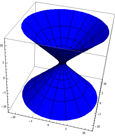
test hyperboloid, a surface of negative Gaussian curvature
signgccolor[{Cos[u] Cosh[v], Sin[u] Cosh[v], Sinh[v]}, {u, 0, 2 Pi}, {v, -Pi, Pi}]


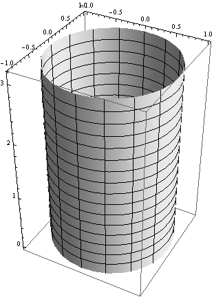
test cylinder, a surface of zero Gaussian curvature
signgccolor[{Cos[u], Sin[u], v}, {u, 0, 2 Pi}, {v, 0, Pi}]


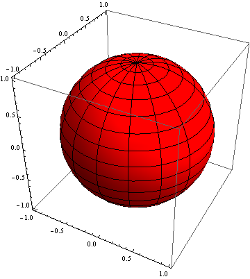
test sphere, a surface of positive Gaussian curvature
signgccolor[{Cos[u] Sin[v], Sin[u] Sin[v], Cos[v]}, {u, 0, 2 Pi}, {v, 0, Pi}]
Posted 10 years ago
Thanks a lot, That really helped,
Is there any way to blend the colors? I mean let the Gaussian curvature of two points like P1 and P2 be m and n where m > n, is it possible to draw P1 darker red if its curvature is positive and likewise lighter blue if its curvature is negative ?
POSTED BY: Ali Noroozi
Reply to this discussion
Community posts can be styled and formatted using the Markdown syntax.
Reply Preview
Attachments
Remove
or Discard

Group Abstract Group Abstract