I recently stumbled upon Three Classes of Newtonian Three-Body Planar Periodic Orbits. Here's a quick way to reproduce their findings using NBodySimulation.

periodic3Body2D[vx0_, vy0_, T_, opts : OptionsPattern[NBodySimulation]] :=
 Block[{x10, y10, x20, y20, x30, y30, vx10, vy10, vx20, vy20, vx30, vy30},
  x10 = -1;
  x20 = 1;
  x30 = 0;
  y10 = y20 = y30 = 0;
  vx10 = vx20 = vx0;
  vx30 = -2 vx0;
  vy10 = vy20 = vy0;
  vy30 = -2 vy0;
  NBodySimulation["InverseSquare", {
    <|"Mass" -> 1, "Position" -> {x10, y10}, 
     "Velocity" -> {vx10, vy10}|>,
    <|"Mass" -> 1, "Position" -> {x20, y20}, 
     "Velocity" -> {vx20, vy20}|>,
    <|"Mass" -> 1, "Position" -> {x30, y30}, 
     "Velocity" -> {vx30, vy30}|>
    }, T, opts]
  ]

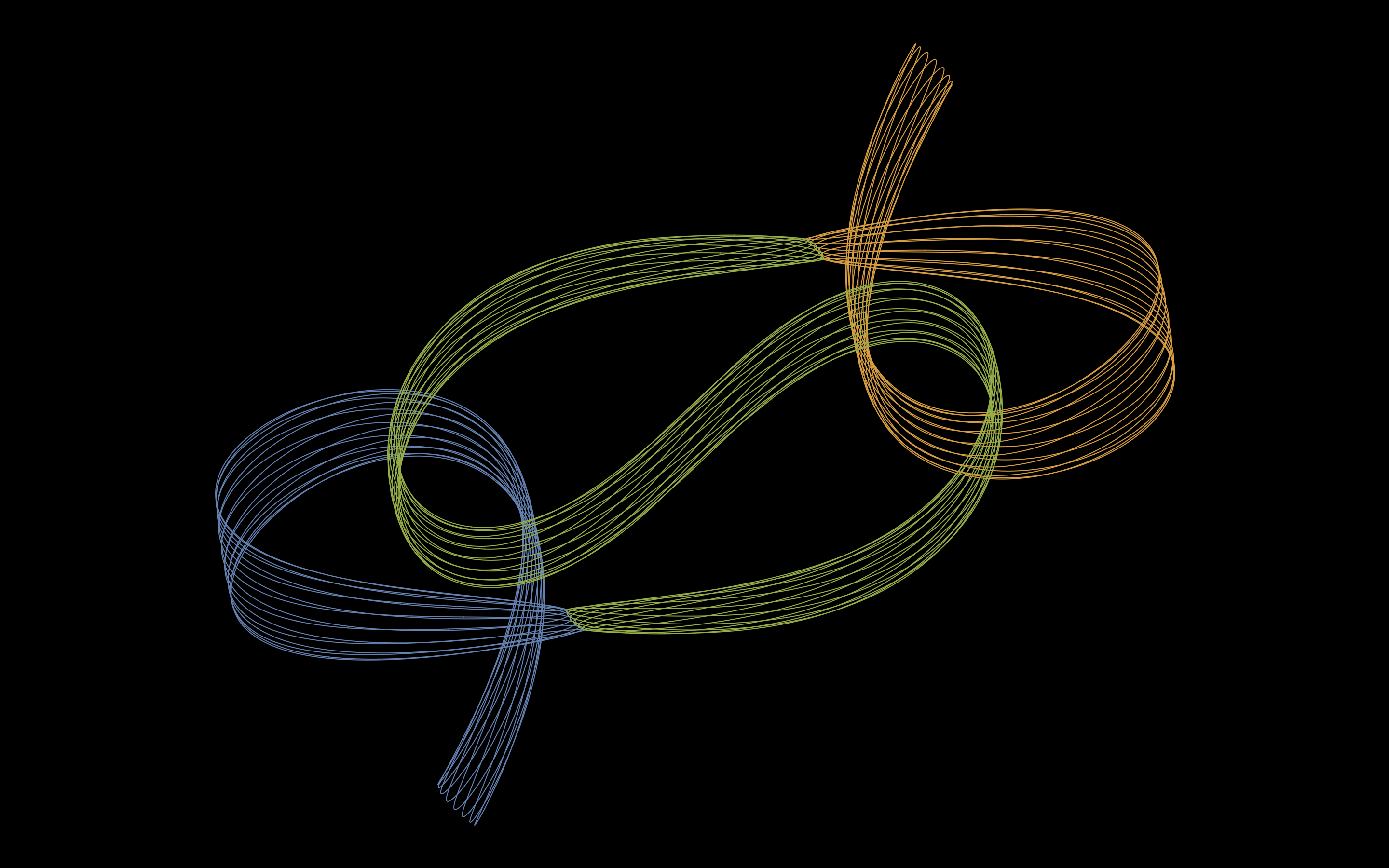
Here's a plot of the full paths of one orbit group listed in the paper:

{vx0, vy0, T} = {0.41682, 0.33033, 55.7898};

yinyangII = periodic3Body2D[vx0, vy0, T, MaxStepSize -> .001];

plot = ParametricPlot[Evaluate[yinyangII[All, "Position", t]], {t, 0, 55.7898}, 
   PlotPoints -> 100, PlotStyle -> AbsoluteThickness[1], 
   Background -> Black, Axes -> False, ImageSize -> 1024, 
   MaxRecursion -> 13] /. Line -> BSplineCurve

Let's write a helper function to plot the three bodies with a trailing orbit at a given time.

First let's find the position of each body at an arbitrary time t. Here we add the capability of sampling over any time point injecting Mod:

bodyPos = yinyangII[All, "Position", t] /. t -> Mod[t, T];

Next, for each body we'll sample from t-1 to t to form a trail. We'll make each vertex in the trail more transparent the closer to t-1 it is. We also represent each body as a point. The use of Transpose ensures the points lie on top of all trails, which comes in handy during a close encounters.

makeFrame[Ts_] :=
  Graphics[
    Transpose@Table[
      With[{c = ColorData[97, i], vals = Table[Evaluate@bodyPos[[i]], {t, Ts - 1, Ts, .001}]},
        {
          {Thick, Line[vals, VertexColors -> Thread[Append[c, Range[0., 1, .001]]]]},
          {PointSize[Large], c, Point[vals[[-1]]]}
        }
      ],
      {i, 3}
    ],
    Axes -> False,
    Background -> Black,
    PlotRange -> {{-1.09, 1.09}, {-0.89, 0.89}},
    PlotRangePadding -> Scaled[.05]
  ]

Here's the configuration at time t == 21:

This could make for a nice screensaver. Let's make a 60 second 10 fps gif:

framecnt = 600;

frames = Monitor[
  Table[
    Rasterize[makeFrame[Ts]],
    {Ts, Subdivide[0, T, framecnt - 1]}
  ],
  Row[{ProgressIndicator[Ts, {0, T}], " ", Ts/T}]
]; // AbsoluteTiming

(* {220.461, Null} *)

Export["orbital_yinyangII.gif", Most[frames], AnimationRepetitions -> ∞, "DisplayDurations" -> 0.1];