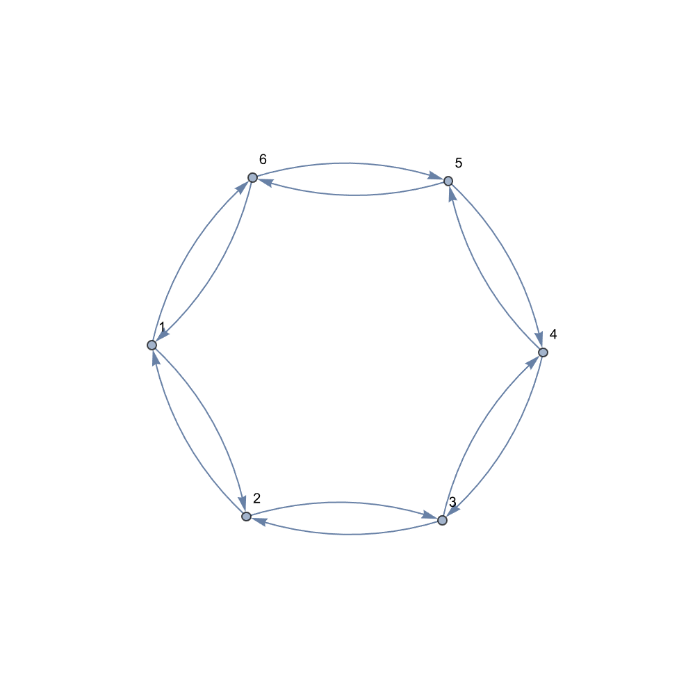
And as you've already illustrated, the computational implementations between cellular automata, perturbations, and the Third Law of Thermodynamics, this is just some additional numerical experiments and visualization techniques that build on the methods you've already described earlier, no changes needed. We already saw that driving a cellular automaton (CA) toward a zero entropy state involves finding the states that naturally evolve to uniformity (or "local consensus")..and then determining the minimum interventions--or perturbations--needed when a CA state is "detached" from the attractive surface. With such interconnected themes, the three themes are as follows..we begin by constructing a transformation matrix for a 6-cell CA, as shown in the code block below. It is this matrix which proposes a linear map whose eigenvalues and associated state graph form an expository analysis of the structural symmetries and connectivity, of the automaton. You can approach that automaton scientifically and a lot of a certain sort of progress is made. I mean I would say that the thing that I'll say over and over again is that: the sort of it. The..it's the "strategy of science" that is much the greatest determiner of scientific success rather than the mechanics of doing the science. The mechanics of doing science is a necessary piece but it's far from a sufficient piece. It's pretty much impossible to do leading edge physics without knowing a certain amount mechanically about 20th century physics and about how to do calculations into 20th century physics and so on and I'd like to think about the tools like Mathematics in Wolfram Language that allow you to do those calculations. The piece that you sort of need is the strategy of what you should study. Let's create a new notebook. It turns out that strategy effectively does what we must; the eigenvalue spectrum reveals fundamental properties of the CA's circulant structure for nearest-neighbor interactions in larger systems & directly relates to the shift invariance observed in the evolution of basis states.
ruleTransformation = {{0, 1, 0, 0, 0, 1}, {1, 0, 1, 0, 0, 0}, {0, 1,
    0, 1, 0, 0}, {0, 0, 1, 0, 1, 0}, {0, 0, 0, 1, 0, 1}, {1, 0, 0, 0,
    1, 0}};
length = Dimensions[ruleTransformation][[1]];
edge = Flatten[
   Table[If[ruleTransformation[[i, j]] == 1, i -> j, Nothing], {i,
     length}, {j, length}]];
graph = Graph[edge, VertexLabels -> "Name", ImagePadding -> 20,
   ImageSize -> 300];
initialState = RandomInteger[{0, 1}, length];
customCA[init_, steps_, noise_] :=
  Module[{state = init, history},
   history =
    Table[state = Mod[state + ruleTransformation . state, 2];
     state =
      Mod[state + RandomVariate[BernoulliDistribution[noise], length],
        2];
     state, {steps}];
   Prepend[history, init]];
evolution = customCA[initialState, 50, 0.1];
Manipulate[
 Grid[{{Graph[edge, VertexLabels -> "Name", ImageSize -> 300,
     VertexStyle ->
      Table[i -> If[evolution[[t, i]] == 1, Red, Blue], {i, length}]],
     ArrayPlot[evolution[[1 ;; t]],
     ColorRules -> {1 -> Red, 0 -> Blue}, Frame -> False,
     ImageSize -> 37]}}], {t, 1, Length[evolution], 1,
  Appearance -> "Labeled"}, ControlPlacement -> Top]
This formalism not only supports the analytics methods for linear automata but also paves the way to advancing our understanding of why linear rules can often be "skipped ahead" computationally. With noise and rule variations moving beyond strictly linear systems, the next set of experiments introduces random noise and allows for rule selection from a "left handed" point of view. Let's evolve an initial binary state using a combination of customCA and a linear update (for example, Rule 150) and a controlled random perturbation. The following is an illustration of a visualization where the evolution, noise level and even the rule type..can be altered on the fly.
n = 30;
length = n;
ruleTransformation =
  Table[If[Mod[j - i, n] == 1 || Mod[i - j, n] == 1, 1, 0], {i,
    n}, {j, n}];
evals = Eigenvalues[ruleTransformation];
entropyL[list_] := Module[{probs}, probs = Counts[list]/Length[list];
   -Sum[probs[[i]]  Log2[probs[[i]]], {i, Length[probs]}]];
customCA[init_, steps_, ruleChoice_] :=
  Module[{state = init, history},
   history =
    Table[state =
      Switch[ruleChoice, "Rule90", Mod[ruleTransformation . state, 2],
        "Rule150",
       Mod[state + ruleTransformation . state, 2]], {steps}];
   Prepend[history, init]];
Manipulate[
 Module[{ca, entropyData}, ca = customCA[init, steps, ruleChoice];
  entropyData = Map[entropyL, ca];
  Column[{Pane[
     ArrayPlot[Transpose[ca], ColorRules -> {0 -> White, 1 -> Black},
      PlotLabel -> Style["CA Evolution", 14, Bold]], {300,
      Automatic}],
    ListPlot[entropyData,
     PlotLabel -> Style["Entropy Over Time", 14, Bold],
     ImageSize -> 300, Filling -> Axis, PlotTheme -> "Scientific"],
    ListPlot[ReIm /@ evals,
     PlotLabel ->
      Style["Eigenvalues (Real \[FilledDiamond], Imaginary \
\[FilledCircle])", 14, Bold], ImageSize -> 300,
     PlotMarkers -> {"\[FilledDiamond]", "\[FilledCircle]"},
     PlotTheme -> "Scientific"]}]], {{ruleChoice, "Rule90",
   "Rule Type"}, {"Rule90", "Rule150"},
  ControlType -> SetterBar}, {{steps, 10, "Simulation Steps"}, 1, 300,
   1, Appearance -> "Labeled"}, {{init,
   Join[{1}, ConstantArray[0, length - 1]]}, ControlType -> None},
 Button["New Initial State", init = RandomInteger[{0, 1}, length],
  ImageSize -> Medium], ControlPlacement -> Top,
 TrackedSymbols :> {ruleChoice, steps, init}]
And that's sort of a necessary piece but the piece of what you need is the strategy of what you should study. People talk about superintelligence, will AIs be the next generation of scientists and so on? Why other people don't think that's a different world, I spent my life building tools that let me to the implementation of the idea as easily as possible. If you can conceptualize something computationally, you've got the fastest path to implement it and see what the consequences of what you've implemented actually are. What am I actually spending my time doing? Well, I'm spending my time thinking about what should I actually do? The mechanics of it have been minimized, because I built Wolfram Language..go from what I think about to type type type and three minutes later, I'm seeing what the consequences of that thought were and it's up to me to think about what do I think about next? And then I'm scratching my head thinking about how to solve the problem but at the scale of actually doing the science, it's really to the point where I'll kind of do something and it'll be fiddley and there will be bugs in the code and so on.
Here, the noise versus deterministic evolution serves as a numerical analogue for "imperfect cooling" in thermodynamic systems. Even small perturbations can lead to divergent trajectories, starting us on the way to drive a system to absolute order--a central tenet of the Third Law.
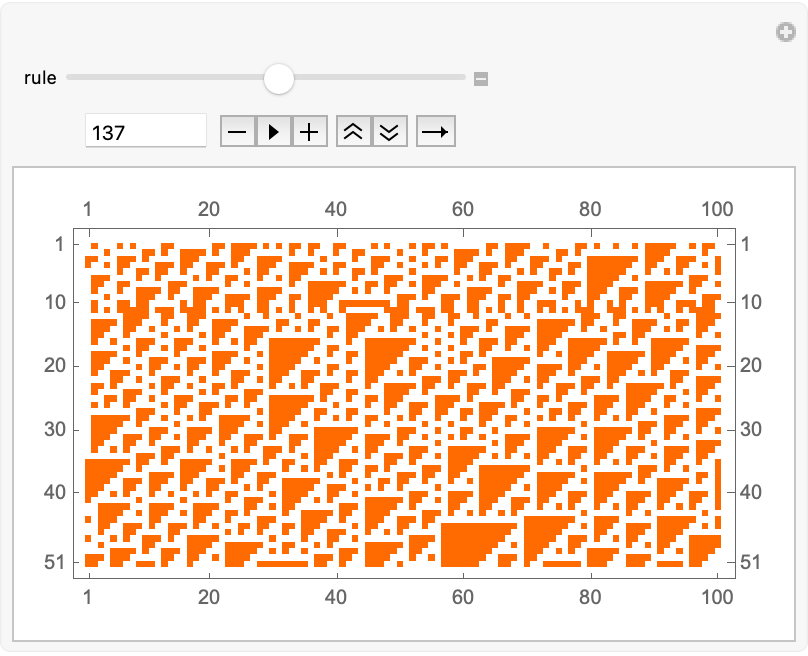
DynamicModule[{init = RandomInteger[{0, 1}, 100], rule = 62,
  initSize = 100, steps = 50,
  ruleTransformation = {{0, 1, 0, 0, 0, 1}, {1, 0, 1, 0, 0, 0}, {0, 1,
      0, 1, 0, 0}, {0, 0, 1, 0, 1, 0}, {0, 0, 0, 1, 0, 1}, {1, 0, 0,
     0, 1, 0}}},
 Column[{Row[{Dynamic[
      Module[{evals, data}, evals = Eigenvalues[ruleTransformation];
       data = Table[{i, Abs[evals[[i]]]}, {i, Length[evals]}];
       ListPlot[data, PlotStyle -> {Red, PointSize[Large]},
        Epilog -> {Orange,
          Table[Line[{{i, 0}, {i, Abs[evals[[i]]]}}], {i,
            Length[evals]}]}, PlotLabel -> "Absolute Eigenvalues",
        AxesLabel -> {"Index", "Magnitude"}, ImageSize -> 200,
        PlotRange -> All]]], Spacer[20],
     Dynamic[ArrayPlot[{init}, ColorRules -> {0 -> White, 1 -> Black},
        PlotLabel -> "Initial Condition", ImageSize -> 300,
       FrameTicks -> Automatic]]}], Spacer[20],
   Manipulate[
    Module[{ca, entropyData, caPlot, entropyPlot, rotatedEntropyPlot},
      ca = CellularAutomaton[rule, init, steps];
     entropyData = Map[entropyL, ca];
     caPlot =
      ArrayPlot[ca, ColorRules -> {0 -> White, 1 -> Black},
       PlotLabel -> "Cellular Automaton Evolution",
       ImageSize -> {300, 300}, FrameTicks -> Automatic];
     entropyPlot =
      ListLinePlot[entropyData, PlotLabel -> "Entropy Evolution",
       AxesLabel -> {"Time", "Entropy"}, ImageSize -> {300, 300},
       Filling -> Axis, PlotRange -> All, PlotStyle -> Purple];
     rotatedEntropyPlot = Rotate[entropyPlot, -Pi/2];
     Grid[{{caPlot, rotatedEntropyPlot}}, Spacings -> {2, 2},
      Alignment -> Center]], {{rule, 62, "CA Rule"}, 0, 62, 1,
     Appearance -> "Labeled"}, {{initSize, 100, "Initial Size"}, 10,
     100, 1, Appearance -> "Labeled"}, {{steps, 50, "Time Steps"}, 10,
      200, 1,
     Appearance ->
      "Labeled"}, {{ruleTransformation, {{0, 1, 0, 0, 0, 1}, {1, 0, 1,
         0, 0, 0}, {0, 1, 0, 1, 0, 0}, {0, 0, 1, 0, 1, 0}, {0, 0, 0,
        1, 0, 1}, {1, 0, 0, 0, 1, 0}}}, ControlType -> InputField,
     FieldSize -> {40, 6}},
    Button["New Initial Condition",
     init = RandomInteger[{0, 1}, initSize], ImageSize -> Medium],
    ControlPlacement -> Left, Paneled -> True, FrameMargins -> 0]}]]
What about when you look at a CA rule and it's supposed to be linear but it's not? Those non-linear CA rules are the ones where you're building a website and it's scaling. In this scenario, no one can quite figure out how the dynamos are governed and they're probably governed by computational irreducibility. And I say probably because if we had the concept of an attractive surface--a collection of states that eventually evolve to a zero entropy configuration--then we wouldn't be examining the Hamming distances between the current state and those in the attractive surface. One can decide on the minimal set of cell flips (perturbations) required. So I eventually found multiple iterations of the attractive surface (or n-iter-dimensional attractive surfaces), why that is is because we iteratively build our ability to predict when and how a perturbation will efficiently "connect" a state to the zero-entropy basin. However, as @Gianmarco Morbelli has already explained, this iterative approach comes at what cost, the cost of rapidly increasing computational demands--a vivid reflection of the Third Law's prescription that zero entropy is only attainable asymptotically.
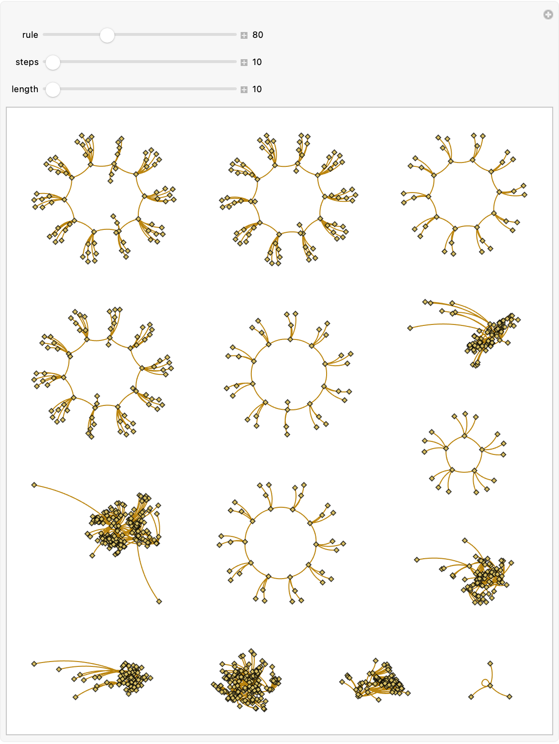
ruleTransformation = {{0, 1, 0, 0, 0, 1}, {1, 0, 1, 0, 0, 0}, {0, 1,
0, 1, 0, 0}, {0, 0, 1, 0, 1, 0}, {0, 0, 0, 1, 0, 1}, {1, 0, 0, 0,
1, 0}}
lenngth = Dimensions[ruleTransformation][[1]];
Eigenvalues[ruleTransformation]
edge = {};
Do[Do[If[ruleTransformation[[i, j]] == 1,
AppendTo[edge, i -> j]],
{j, 1, lenngth}] ,
{i, 1, lenngth }]
Graph[edge,
VertexLabels -> "Name",
ImagePadding -> 100,
ImageSize -> 500]
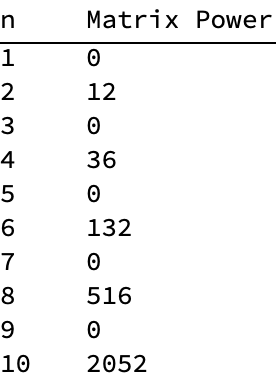
TableForm[
Table[{n, Tr[MatrixPower[ruleTransformation, n]]}, {n, 10}],
TableHeadings -> {None, {"n", "Matrix Power"}}]
Therefore the evolution of the matrix..
What about people like me who don't even know any binary? That must be why the Third Law requires an infinite amount of steps in its definition.
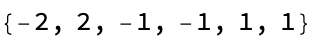
Reading your article is like reading the textbook; the cellular automata evolution is like that. Do you want to choose a perturbation? The Third Law of Thermodynamics, when transposed to the "realm" of cellular automata, is not merely an abstract statistical statement but a direct implication of computational irreducibility. The necessity of infinite or impractically large sequences of well-timed perturbations to force a Cellular Automaton into a zero entropy state encompasses the intrinsic limitations in our motivations to "cool" complex computational systems. The general non-linear case resists such simplifying analytical shortcuts which while they do exist for additive systems, it's just another echo chamber spanning the thematic canvas of irreversibility and the practical unattainability of absolute order. Ciao..computational techniques of ours that's being further minimized. I'll ask the notebook assistant and it usually gives me a good idea about how to do it even if it doesn't slam dunk solve it. In terms of the formalism that we had at the time..doesn't need much updating.
Manipulate[
 Module[
  {init = RandomInteger[1, length], transs},
  transs =
   GraphPlot[# -> CellularAutomaton[rule, #] & /@
     Tuples[{0, 1}, length],
    DirectedEdges -> True,
    GraphStyle -> "Prototype",
    GraphLayout -> "SpringEmbedding",
    EdgeShapeFunction -> "CurvedArc",
    VertexShapeFunction -> "Diamond"];
  Grid[{{transs}}]],
 {rule, 0, 255, 1, Appearance -> "Labeled"},
 {steps, 10, 100, 1, Appearance -> "Labeled"},
 {length, 10, 100, 1, Appearance -> "Labeled"}]
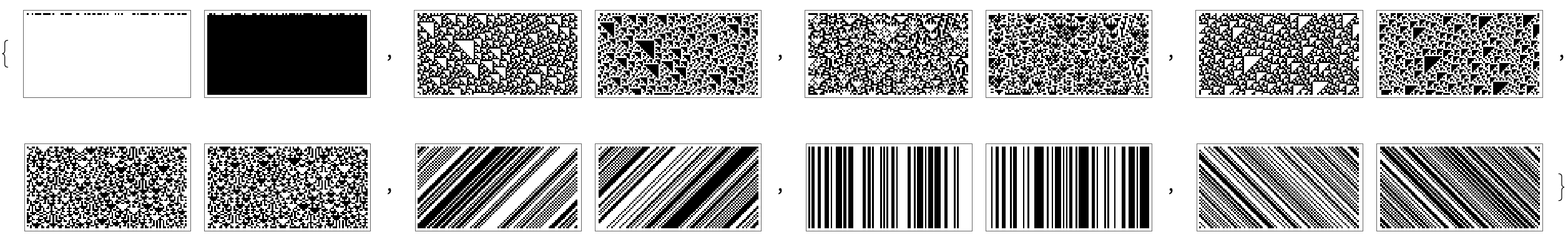
The third law of thermodynamics, within the context of computational programs: cellular automata..let's do a computational walk through the complex behavior, of physical systems. That part went way, over my head and I was afraid to ask. Soo, the third law of thermodynamics states that whensince reducing the entropy of a system to absolute zero.. a measure of randomness or disorder..maybe there's a way to explore the way that cellular automata are traditionally..defined. When we create some "vigorous" perturbations in the cellular automata that is temporary changes in cell states..we can try and drive the system towards a state of minimum entropy and then..all cells are the same color. If that's our state of minimum entropy, here's how to reach local consensus.
SeedRandom[561];
swapSimple[rule_, init_, t_] := 1 - CellularAutomaton[rule, init, t]
plotComparison[rule_, init_, t_] := GraphicsRow[{
   ArrayPlot[CellularAutomaton[rule, init, t]],
   ArrayPlot[swapSimple[rule, init, t]]
   }, ImageSize -> 300]
linearRules = {0, 60, 90, 102, 150, 170, 204, 240};
plotComparison[#, RandomInteger[1, 100], 50] & /@ linearRules
Computational implications of the third law of Thermodynamics is all very beautiful and I am very happy to be able to represent this concept within the cellular automata, linear and non-linear. Linear automata, an analytical method developed to find the set of states that evolve to a zero state..involved finding the kernel of the transformation rule for the automata. How do I solve the kernel? Here is the best explanation of how to solve things..
substituteCellularAutomata[rule_, init_, t_, sub_] :=
With[{subList =
Flatten[Join[ConstantArray[rule, sub[[2]] - 1],
PadRight[{#1}, #2, rule] & @@@
Partition[
Riffle[sub[[;; ;; 2]], (#2 - #1) & @@@
Partition[Join[sub, {rule, t + 1}][[2 ;; ;; 2]], 2, 1]],
2]], 1]},
FoldList[CellularAutomaton[#2, #1, {{{1}}}] &, init, subList]]
init = RandomInteger[1, 50];
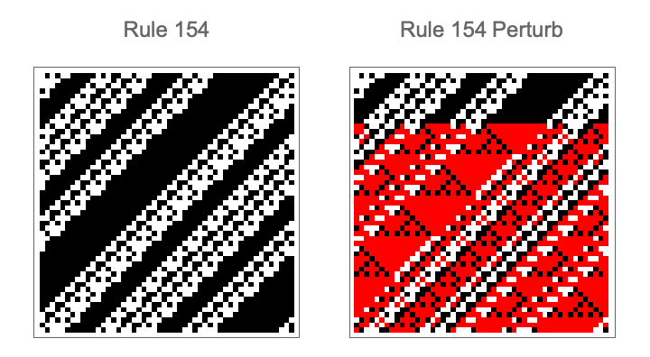
rule = 154;
perturbPlot =
MapAt[Red &,
substituteCellularAutomata[rule, init,
50, {{Mod[#[[1]] + #[[3]], 2] &, {}, 1}, 10}],
Position[
Partition[
MapThread[
Equal, {Flatten[
substituteCellularAutomata[rule, init,
50, {{Mod[#[[1]] + #[[3]], 2] &, {}, 1}, 10}]],
Flatten[CellularAutomaton[rule, init, 50]]}], 50], False]];
GraphicsRow[{ArrayPlot[CellularAutomaton[rule, init, 50],
PlotLabel -> "Rule " <> ToString[rule]],
ArrayPlot[perturbPlot,
PlotLabel -> "Rule " <> ToString[rule] <> " Perturb"]},
ImageSize -> Medium]
Hmm..remove duplicates to find the states unique that evolve to zero. But that's just how I see it. But then I can identify these states and develop a function to find the cell perturbations, the minimum number needed to drive the automata to a zero state? This is it, this is the one-point crossover. I really enjoyed exploring the concept of the "attractive surface" that, after a certain number, what is it? I don't know..the iterations, break them down into 1-iter dimensional attractive surfaces.
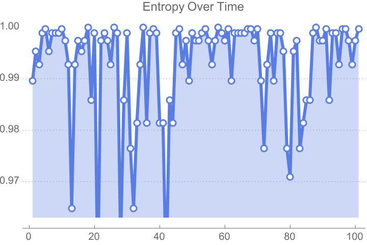
entropyL[list_] := Module[
  {probs},
  probs = Counts[list]/Length[list];
  -Sum[probs[[i]] Log2[probs[[i]]], {i, Length[probs]}]
  ]
plotEntropy[rule_, init_, t_] := ListLinePlot[
  Map[entropyL, CellularAutomaton[rule, init, t]],
  PlotLabel -> "Entropy Over Time",
  AxesLabel -> {"Time", "Entropy"},
  ImageSize -> Medium,
  Filling -> Axis,
  PlotTheme -> "Business"]
init = RandomInteger[1, 100];
plotEntropy[30, init, 100]
Let's say we want to highlight how the Third Law of Thermodynamics implications play out, in computational models, through the cellular automata lens. Focus on the non-linear behavior with a focus on their "attractive surfaces". And those are the states, that we do evolve to zero entropy states. We don't need to distinguish between states that we visually represented with transition diagrams..these weren't even connected to the attractive surface. Supposedly it's possible to analyze this exquisite evolution of these states via Hamming entropy that makes most states stabilize, what did you expect, at a fixed Hamming distance from the periodic behavior display.
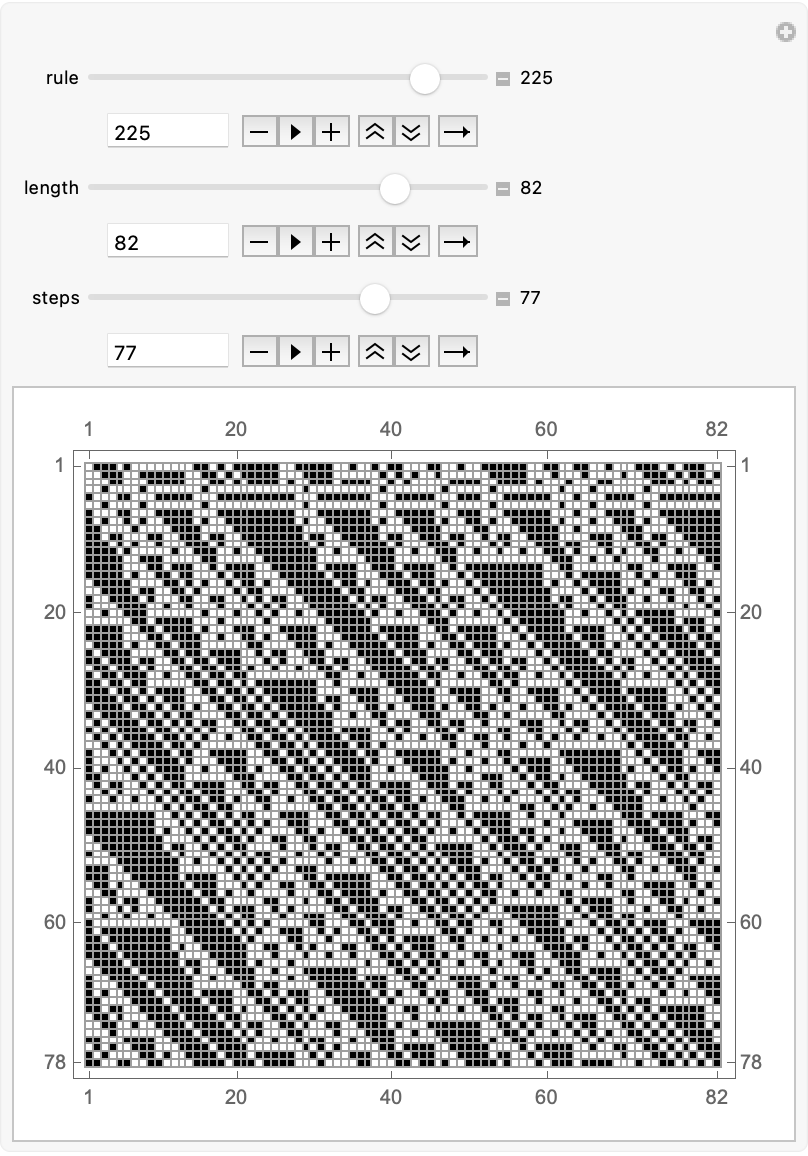
Manipulate[
 Module[
  {init = RandomInteger[1, length]},
  MatrixPlot[
   substituteCellularAutomata[rule, init, steps, {2, 3, 1, 5}],
   Mesh -> True,
   FrameTicks -> All,
   ColorFunction -> "Monochrome"]],
 {rule, 0, 255, 1, Appearance -> "Labeled"},
 {length, 10, 100, 1, Appearance -> "Labeled"},
 {steps, 10, 100, 1, Appearance -> "Labeled"}]
@Gianmarco Morbelli implements a function that identifies which state within the evolution comes closest to the attraction surface states, and applies the perturbations necessary to this state in the right sequence to drive the cellular automata to a zero entropy state, visually represented in a transition diagram, and highlights the role of the perturbation in connecting two disconnected regions of the state graph.
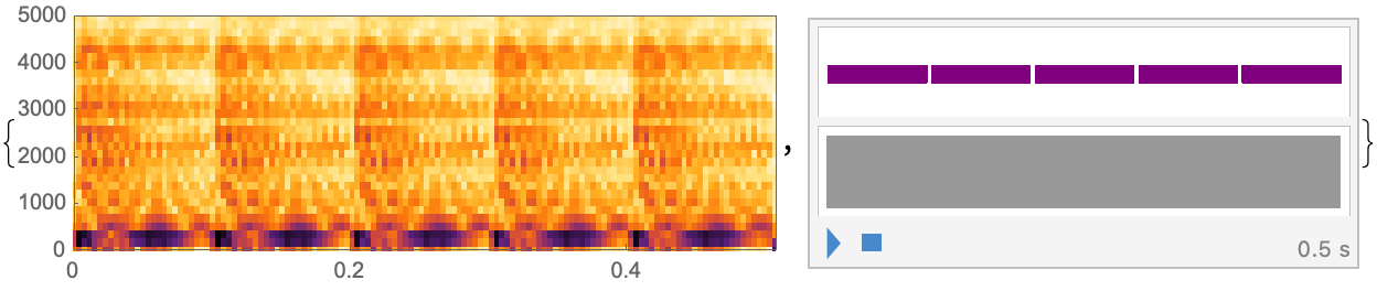
automatonSpectrogram[rules_, inits_, steps_] := Module[
  {automatons, sound, instrument = "Piano"},
  automatons =
   MapThread[
    substituteCellularAutomata[#1, #2, steps, {2, 3, 1, 5}] &, {rules,
     inits}];
  sound = Sound[
    Flatten[
     MapThread[
      SoundNote[#1, 0.1, instrument] &,
      {Mod[Flatten[#], 88] & /@ automatons}]]];
  {Spectrogram[sound, ImageSize -> 345], sound}]
automatonSpectrogram[{90, 30, 110, 45, 210},
 RandomInteger[1, {5, 50}], 12]
@Gianmarco Morbelli I want to do update the function, add in the attractive surfaces states that map to the zero state after some n iterations...increasing the computational effort required while reducing all these perturbations needed to reach the zero state, and this perturbation provides valuable insights into the computational models, the study of thermodynamics..why not introduce a "update" to achieve zero entropy states?
Manipulate[init = RandomInteger[1, 100];
 t = 50;
 sub = {RandomInteger[{0, 255}], 10, RandomInteger[{0, 255}], 11};
 g = substituteCellularAutomata[rule, init, t, sub];
 MatrixPlot[g], {rule, 0, 255, 1}]
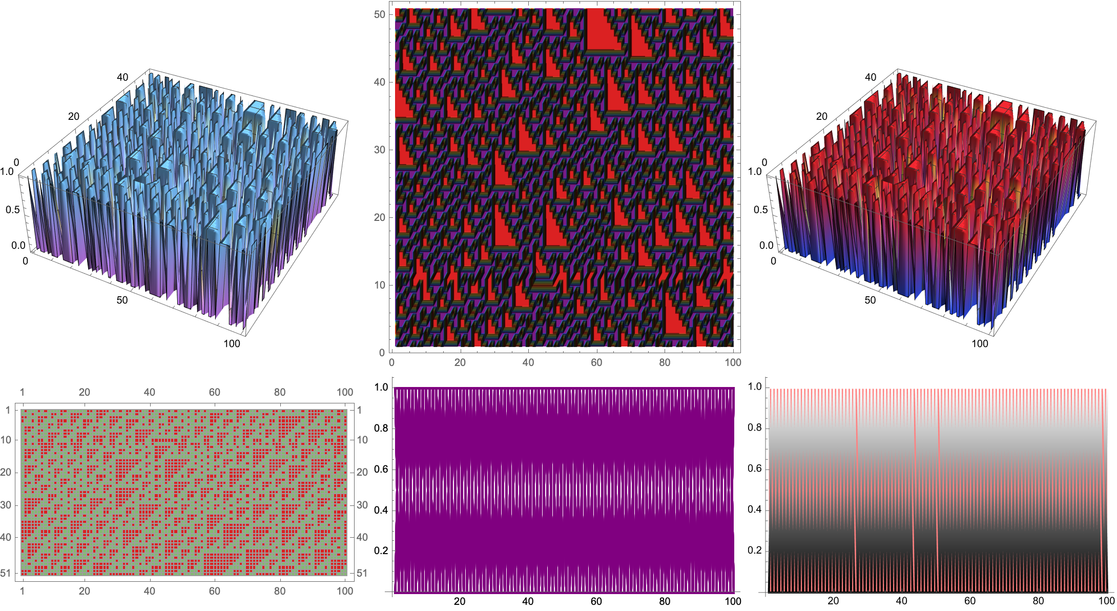
Alright, that's enough. At the procedure..after all, driving cellular automata to a zero entropy state requires finding the states that do evolve to the zero state after an arbitrary number of iterations..which, results in a significance in computational effort. With that I hope you are doing well, as the nearest person to our customer, our next of kin. Besides, it's the result that we've been waiting for: as the number of cells increases, it becomes unfeasible computationally to predict the states contained within the attractive surfaces..this really checks all the right boxes. It's not just the instance of computational irreducibility, or the lack of information, or the inability to determine what perturbations to apply to reach a state of zero entropy, it's the Third Law of Thermodynamics.
Grid[{{ListPlot3D[g, ColorFunction -> "Pastel", ImageSize -> Medium],
   ListContourPlot[g, ColorFunction -> "Rainbow",
    ImageSize -> Medium],
   ListPlot3D[g, ColorFunction -> "TemperatureMap",
    ImageSize -> Medium]}, {MatrixPlot[g, ColorFunction -> "Rainbow",
    Mesh -> True, ImageSize -> Medium],
   ListLinePlot[substituteCellularAutomata[30, init, t, sub],
    PlotStyle -> Directive[Purple, Thick], ImageSize -> Medium],
   ListLinePlot[g, ColorFunction -> "SunsetColors",
    PlotStyle -> Directive[LightBlue, Thick], Filling -> Axis,
    FillingStyle -> Pink, ImageSize -> Medium]}}]
That's the Third Law, It's impossible or difficult to reach a state of zero entropy without infinite steps. This reflects the infinite trials needed, to find the correct perturbations. The Second Law of Thermodynamics deals with the decrease of entropy..or the impossibility of finding initial conditions that leads to the decrease in entropy. I'm just out here in these interpretations, perturbations applying the Knuth-Bendix algorithm for rewriting systems, where the perturbations would be interpreted..as performing completions on a graph to reach local confluence and test the consequences, thermodynamically. Understanding any specific mathematical formalism is like understanding binary; understanding binary is not crucial to understanding the Third Law. In its definition, there is no necessity other than to reflect the computational irreducibility and complexity in here in this system and suggests that the laws of thermodynamics are all connected to the principles, of computational irreducibility.


