I think the best Q & A that we did (Questions & Answers..spell it out cause that's probably the best use of Wolfram Language Code)..you've definitely shown us some ways that we can expand upon our high-school-level International Baccalaureate Diploma Programme. To understand this, these "practical" demonstrations lead us to reflections in broad brush-strokes on efficiency, computational innovation, and career pathways, as these are the reasons why we combine subject-matter mastery and all things central to productive calculus teaching. Everybody knows that these are the questions we should be asking, whether it's the creativity that serves as the foundation of efficient workflow and I know this is stuff we've already seen before. Well, that might be familiar to teachers & educators who are steeped in such an environment but, it might not be familiar to the "uninitiated" which is why it takes so long to process all these Wolfram Demonstrations. The following is a "snippet" of Wolfram Language code that provides a brief introduction to the fundamentals of mathematical illustration.

ClearAll["Global*"];
Manipulate[
 Module[{f1, f2, f3, f4, df1, df2, df3, df4, aVal, t1, t2, t3, t4, 
   xRange, yRange}, f1 = Sin[x];
  f2 = Cos[x];
  f3 = x^3 - 3  x;
  f4 = Exp[-x/3]*Sin[2  x];
  df1 = D[f1, x];
  df2 = D[f2, x];
  df3 = D[f3, x];
  df4 = D[f4, x];
  aVal = a;
  t1 = (f1 /. x -> aVal) + (df1 /. x -> aVal)*(x - aVal);
  t2 = (f2 /. x -> aVal) + (df2 /. x -> aVal)*(x - aVal);
  t3 = (f3 /. x -> aVal) + (df3 /. x -> aVal)*(x - aVal);
  t4 = (f4 /. x -> aVal) + (df4 /. x -> aVal)*(x - aVal);
  xRange = {-3, 3};
  yRange = {-3, 3};
  Grid[{{Plot[{f1, t1, f2, t2, f3, t3, f4, t4}, {x, xRange[[1]], 
       xRange[[2]]}, PlotRange -> {yRange, Automatic}, 
      PlotStyle -> {Directive[Thick, Blue], 
        Directive[Thick, Blue, Dashed], Directive[Thick, Red], 
        Directive[Thick, Red, Dashed], Directive[Thick, Purple], 
        Directive[Thick, Purple, Dashed], Directive[Thick, Black], 
        Directive[Thick, Black, Dashed]}, 
      Epilog -> {{Blue, PointSize[0.02], 
         Point[{aVal, f1 /. x -> aVal}]}, {Red, PointSize[0.02], 
         Point[{aVal, f2 /. x -> aVal}]}, {Purple, PointSize[0.02], 
         Point[{aVal, f3 /. x -> aVal}]}, {Black, PointSize[0.02], 
         Point[{aVal, f4 /. x -> aVal}]}}, AxesLabel -> {"x", "y"}, 
      PlotLabel -> Style["Functions and Tangent Lines", 14, Bold], 
      ImageSize -> 400], 
     Plot[{df1, df2, df3, df4}, {x, xRange[[1]], xRange[[2]]}, 
      PlotRange -> {yRange, Automatic}, 
      PlotStyle -> {Thick, Thick, Thick, Thick}, 
      Filling -> 
       If[showDerivArea, {1 -> Axis, 2 -> Axis, 3 -> Axis, 4 -> Axis},
         None], FillingStyle -> Directive[Opacity[0.2]], 
      Epilog -> {{Blue, PointSize[0.02], 
         Point[{aVal, df1 /. x -> aVal}]}, {Red, PointSize[0.02], 
         Point[{aVal, df2 /. x -> aVal}]}, {Purple, PointSize[0.02], 
         Point[{aVal, df3 /. x -> aVal}]}, {Black, PointSize[0.02], 
         Point[{aVal, df4 /. x -> aVal}]}}, AxesLabel -> {"x", "y'"}, 
      PlotLabel -> Style["Derivative Functions", 14, Bold], 
      ImageSize -> 400]}}]], {{a, 0, "Tangent point (a)"}, -3, 3, 0.1,
   Appearance -> "Labeled"}, {{showDerivArea, True, 
   "Show derivative area"}, {True, False}}, 
 SynchronousUpdating -> False]

Here you will find four different functions--sine, cosine, a cubic polynomial, and a damped sinusoid--AND their derivatives. The "idea" underneath is that the user can drag a slider to set a "tangent point" α, and mathematically draw both the function & its tangent line algebraically & automatically. On the right, you see each function's derivative plotted, with an alternate type of shading area around each and every derivative. I mean so what if we have to check the box every time it's so much better than manually shading. As a side note I recently attended a lecture series called Navigating Academia Under the Patriarchy by The Diversity in Biological Sciences Council at Northwestern University. There..we had a guest speaker who remarked specifically on the concept of how to increase a teacher's efficiency, under the patriarchy. The key takeaway is that we have to find bubbles of time to do research, which requires efficiency. Can you think of any ways to make Mathematica any more efficient than it already is? Now, we get to spend a significant amount of time doing these things. Part of the reason for that is that I think we've managed to become fairly efficient in our lives. Efficiency might seem like an over-generalization, of the value of time-management. But the utility of the Wolfram Language has become the ultimate computational tool for time management; having access to these tools significantly boosts a teacher's efficiency. Instead of manually computing multiple tangents and derivatives and blanking out, one like-wise can rely fully and completely on this dynamic auto-updating type of plot. This extra efficiency is a great setup because more time can be promptly dedicated to even greater things like class discussions! How does a derivative represent the rate of change? Why is the tangent line a better and better approximation as Δx→0? These tools, help reclaim precious time for research and exploration. As we used to say, back in the day being "efficient enough" to focus on what really matters is key to innovation. A lot of us struggle with cultivating a research mindset. I think that our success in blending and mushing together interactive learning with research not only enriches the classroom experience but also prepares the next generation of thinkers to be ready to tackle complex problems with creativity & efficiency, which demonstrates the profound impact of Wolfram's computational tools on both teaching and research. Cultivating a research mindset--much like the ancient Socratic method--combined with the method of bubbles of creativity, make careers in research the story of an enduring pedagogy foretold. Before we get into more details I would like to more properly introduce the bifurcation diagram as well as something called a Cobweb plot.

bifurcationData = 
  Flatten[Table[
    Module[{rVal = r0, orbit, asymptotic}, f[x_] := r0*x*(1 - x);
     orbit = NestList[f, 0.25, 1000];
     asymptotic = Drop[orbit, 500];
     {r0, #} & /@ asymptotic], {r0, 2.5, 4.0, 0.002}], 1];
Manipulate[
 Module[{orbit, lines}, orbit = NestList[r  #  (1 - #) &, 0.5, 50];
  lines = 
   Flatten[Function[{prev, 
       next}, {{{prev, prev}, {prev, next}}, {{prev, next}, {next, 
         next}}}] @@@ Partition[orbit, 2, 1], 1];
  Grid[{{Plot[{r*x*(1 - x), x}, {x, 0, 1}, 
      PlotRange -> {{0, 1}, {0, 1}}, 
      Epilog -> {{Red, Line[lines], PointSize[0.02], 
         Point[Transpose[{orbit, orbit}]]}, 
        Text[Style["Cobweb Diagram", Bold, 16], {0.5, 1.05}]}, 
      PlotStyle -> {Blue, {Black, Dashed}}, ImageSize -> 400, 
      AspectRatio -> 1, AxesLabel -> {"x", "f(x)"}], 
     Show[ListPlot[bifurcationData, 
       PlotStyle -> {Black, PointSize[0.001]}, 
       PlotRange -> {{2.5, 4.0}, {0, 1}}, ImageSize -> 400, 
       AxesLabel -> {"r", "x"}, 
       Epilog -> 
        Text[Style["Bifurcation Diagram", Bold, 16], {3.25, 1.05}]], 
      Graphics[{{Red, Thickness[0.005], 
         Line[{{r, 0}, {r, 1}}]}, {Dashed, Gray, 
         Line[{{2.5, 0.5}, {4.0, 0.5}}]}}]]}}, Spacings -> 0, 
   Frame -> All]], {{r, 3.0, "Parameter r"}, 2.5, 4.0, 0.01, 
  Appearance -> "Labeled", ControlPlacement -> Top}, 
 TrackedSymbols :> {r}, FrameMargins -> 0]

Here we have some additional logistic maps. Specifically, f(x) = rx(1-x) translates to the Cobweb diagrams (that we see on the left panel) and the famous bifurcation diagram (that we see on the right panel). Students, can learn about period doubling, chaos, and the transition from stable solutions to complex behavior as r increases. What's the connection to the concept of computational practicality? Well, fortunately for us we've got countless heated discussions and Wolfram Demonstrations on the interface between theoretical exploration and practical applications, and thus we shall introduce an example on coffee cooling and some real-world phenomena. It might not change the world but it does utilize tools like the logistic map demonstration; these are the tools which show how quickly simple iterative processes can become complicated--this mirrors the forgotten "unexpected consequences" concept that we explored earlier on. In our research, in previous classrooms we did mention this that yes, if you just define a thing you want, of course there will always be unexpected ways that that might be achieved. Sometimes, the way that students experiment for instance with r from 2.5 to 4.0 just might reveal how quickly unexpected behavior can arise via the foundational simple equation.

ClearAll["Global*"];
f[x_] := 4  Sin[5  x]  Exp[-x/5] + 3;
fprime[x_] = Evaluate[D[f[x], x]];
Manipulate[
 Row[{LocatorPane[Dynamic[{a, f[a]}, (a = #[[1]]) &], 
    Show[Plot[f[x], {x, 0, 20}, PlotStyle -> Directive[Purple, Thick],
       PlotRange -> {{0, 20}, {-1, 7}}, AxesLabel -> {"x", "f(x)"}, 
      PlotLabel -> 
       Style["Function with Tangent and Secant Lines", 16], 
      ImageSize -> 450], 
     Graphics[{{Red, Thick, 
        InfiniteLine[{{a, f[a]}, {a + 1, f[a] + fprime[a]}}]}, {Green,
         Thick, Line[{{a, f[a]}, {a + h, f[a + h]}}]}, {Gray, Dashed, 
        Line[{{a, 0}, {a, f[a]}}]}, {Black, PointSize[0.02], 
        Point[{a, f[a]}]}, 
       Text[Style["Tangent Line", Red, 12], {a + 1, 
         f[a] + fprime[a]}, {-1, 0}], 
       Text[Style["Secant Line", Green, 
         12], {a + h/2, (f[a] + f[a + h])/2}, {0, -1}]}], 
     PlotRange -> All], Appearance -> None], 
   Plot[fprime[x], {x, 0, 20}, PlotStyle -> Directive[Orange, Thick], 
    PlotRange -> All, AxesLabel -> {"x", "f'(x)"}, 
    PlotLabel -> Style["Derivative Function", 16], 
    Epilog -> {{PointSize[0.02], Point[{a, fprime[a]}]}, 
      Text[Style[
        StringForm["f'(1) = 2", Round[a, 0.01], 
         NumberForm[fprime[a], {3, 2}]], 12], {a, fprime[a]}, {0, 
        1.5}]}, ImageSize -> 450]}], {{a, 10, "Tangent Point"}, 0, 20,
   0.1, Appearance -> "Labeled"}, {{h, 0.5, 
   "Secant \[CapitalDelta]x"}, 0.1, 2, 0.1, Appearance -> "Labeled"}, 
 SynchronousUpdating -> False]

What does that mean, to teach IBDP Calculus? For the longest time I couldn't tell whether that was a tangent or a secant slider for a single function..but now as we drag the locator to define the tangent point on f, it turns out also that we can change the secant line offset h..the right panel separately plots the derivative f'(x) and shows its real-time value at x = a which progressively cools off. This development epitomizes the "quick iteration" approach: in which, we can collectively agree that we can see the effect of altering a and h in real-time, saving hours of manual graph-sketching. And, in the International Baccalaureate Calculus computational paradigm, it is this efficiency that really frees the teacher to discuss key ideas--it's really the original limit definition of the derivative that is highly valuable--therefore rather than losing time drawing or revising static plots, we can instead transition from the concept of tangents and secants to Epsilon-Delta reasoning.

Clear["Global*"];
Manipulate[
 Module[{f, df, tanLine, secLine, x1, y1, epsRect, deltaRect}, 
  f[x_] := 
   Switch[func, 1, x^3 - 3  x, 2, Sin[Pi  x], 3, Exp[-x/2]  Sin[3  x]];
  df[x_] = D[f[x], x];
  tanLine[x_] := df[a]  (x - a) + f[a];
  secLine[x_] := (f[a + h] - f[a])/h  (x - a) + f[a];
  {x1, y1} = {a + h, f[a + h]};
  epsRect = {Opacity[0.3], Green, 
    Rectangle[{a - \[Delta], f[a] - \[CurlyEpsilon]}, {a + \[Delta], 
      f[a] + \[CurlyEpsilon]}]};
  deltaRect = {Opacity[0.2], Blue, 
    Rectangle[{a - \[Delta], -10}, {a + \[Delta], 10}]};
  Show[Plot[{f[x], tanLine[x], secLine[x]}, {x, -3, 3}, 
    PlotStyle -> {Directive[Thick, Purple], Directive[Thick, Orange], 
      Directive[Thick, Dashed, Blue]}, 
    PlotRange -> {{-3, 3}, {-3, 3}}, PlotRangePadding -> 0.2, 
    PlotTheme -> "Detailed", Background -> Lighter[Yellow, 0.9], 
    Frame -> True, FrameStyle -> Directive[Black, Thick], 
    FrameLabel -> {Style["x", 14], Style["f(x)", 14]}, 
    PlotLabel -> Style["New Epsilon-Delta Demo", 16, Bold, Blue], 
    PlotLegends -> {Style["f(x)", Purple], Style["Tangent", Orange], 
      Style["Secant", Blue]}, TicksStyle -> Directive[Black, 14], 
    GridLines -> Automatic, GridLinesStyle -> LightGray, 
    ImageSize -> 600, PlotPoints -> 200, PerformanceGoal -> "Quality",
     Epilog -> {{PointSize[0.03], Purple, Point[{a, f[a]}], Blue, 
       Point[{x1, y1}]}, epsRect, 
      deltaRect, {Dashed, Gray, Line[{{a, -3}, {a, 3}}]}}], 
   Graphics[{Text[
      Style[StringForm["f'(a) = `", NumberForm[df[a], {3, 2}]], 18, 
       Orange], {a + 0.5, f[a] + 0.5}]}], PlotRangeClipping -> True]],
  Row[{Control[{{func, 1, "Function"}, {1 -> "x³ - 3x", 
      2 -> "sin(\[Pi] x)", 3 -> "e^(-x/2) sin(3x)"}}], Spacer[20], 
   Control[{{a, 0, "Point of tangency (a)"}, -2.5, 2.5, 0.1, 
     Appearance -> "Labeled"}], Spacer[20], 
   Control[{{h, 1, "Secant offset (h)"}, -2, 2, 0.01, 
     Appearance -> "Labeled"}]}], 
 Row[{Control[{{\[CurlyEpsilon], 0.5, "\[CurlyEpsilon]"}, 0.1, 2, 0.1,
      Appearance -> "Labeled"}], Spacer[20], 
   Control[{{\[Delta], 0.5, "\[Delta]"}, 0.1, 2, 0.1, 
     Appearance -> "Labeled"}]}], 
 TrackedSymbols :> {func, a, h, \[CurlyEpsilon], \[Delta]}, 
 Paneled -> True, FrameMargins -> 0, Alignment -> Center, 
 ControlPlacement -> Top]

I think my favorite Wolfram Demonstration is the Coffee Cooling Problem. Whether it's the syrup or sucralose that you add to your coffee, you have got to consider how such a simple example has its correlates and origins in the Epsilon-Delta Demonstration; here, we transition from the concept of tangents and secants to Epsilon-Delta reasoning. The segue is that a rectangle bounding the function near x_0 is the easiest way of saying that the function stays within Epsilon or some limit or line. Limits and continuity often feel opaque and ritualistic to high-schoolers, who see them in a purely symbolic sense. What we don't know is that while the Wolfram Language looks ritualistic from the outside, it is a fluke of our computational capacity that we can demonstrate this in a bubble in time -- a teacher can allocate a short interactive block in class and let the demonstration handle the grunt work. Wherever you can find that niche you will find a chance to do research, some learning..hopefully contributing good things. Turning on the "Show Tangent Line," for instance or exploring when the function's actual value stays within green Epsilon-bands, fosters a more intuitive grasp of these advanced concepts. Allow me to explain to you another Epsilon-Delta visualization, with Sin(x)/x this time.

It's certainly not animation on par with Pixar but there's definitely some merit to the capacity of these demonstrations to focus on the following:

\begin{cases} f(x) = 1, & x = 0 \ \ \ \ \ \ \ and/or \ \ \ \ \ \ \ f(x) = x \sin x, & x \neq 0 \end{cases}

Forget about the LaTeX snippets now; there's a way to do it in a fastly manner. Here we can show continuity at x = 0 and sin(x) / x→1. And I think the sliders for Epsilon and Delta help show the bounding box around {x_0, f[x_0]}. The gist is that if we do the sliders and the bounding box we'll sometimes be able to tell the behavior, and then we can make some different decision. International Baccalaureate Diploma Programme teachers can adapt that same kind of decision-making logic in the classroom by letting students physically see how bounding intervals define whether the graph is inside or outside the Epsilon range; something that would be more apparent to Wolfram veterans like us might not be so apaprent to educators which is why we need to implement all these code blocks. It doesn't even look like the Wolfram Mathematica code that we're used to, because this is just a subsection of the things that we can do in the conventional sense. So here I present you with the sixth idea for teaching I.B.D.P. Calculus in a way that bypasses the limit at infinity via the decaying sinusoid/rational/exponential.

ClearAll["Global*"];
Manipulate[xmax = 20;
 ymax = 7;
 {selectedFunction, L, limitExpr} = 
  Switch[func, 
   1, {4  Sin[5  x]  E^(-x/5) + 3, 3, 
    HoldForm[4  Sin[5  x]  E^(-x/5) + 3]}, 
   2, {(2  x + 1)/(x + 1), 2, HoldForm[(2  x + 1)/(x + 1)]}, 
   3, {5  E^(-x/2), 0, HoldForm[5  E^(-x/2)]}];
 f[x_] := selectedFunction;
 DynamicModule[{pt = {xxx, L}}, 
  Deploy@Labeled[
    Column[{LocatorPane[
       Dynamic[pt, (pt = {#[[1]], L}; xxx = #[[1]]) &], 
       Deploy@Show[
         Plot[f[x], {x, 0, xmax}, PlotStyle -> Purple, 
          PlotRange -> {{0, xmax}, {-1, ymax}}], 
         Graphics[{{Orange, 
            Line[{{xxx, 0}, {xxx, ymax}}]}, {Lighter[Gray, 0.5], 
            Line[{{0, L}, {xmax, L}}]}, {Darker[Green, 0.5], 
            Line[{{0, L - ep}, {xmax, L - ep}}], 
            Line[{{0, L + ep}, {xmax, L + ep}}]}, {Black, 
            PointSize[0.015], 
            Point[{xxx, 0}]}, {Text[
             Style["M", Italic, 16], {xxx, 0.3}]}, {Text[
             Style["L", Italic, 16], {0.3, L}]}}], 
         PlotRange -> {{0, xmax}, {-1, ymax}}, ImagePadding -> 10, 
         ImageSize -> 400, 
         Ticks -> {Union[Table[{n, n}, {n, 0, xmax}]], 
           Union[Table[{n, n}, {n, 0, ymax}]]}]], 
      Row[{Text@
         Style[Row[{" \[CurlyEpsilon] = ", ep}], 20, 
          Darker[Green, 0.5], Bold], "   ", 
        Text@Style[Row[{Style["M", Italic], " = ", Dynamic[xxx]}], 20,
           Orange, Bold]}]}], 
    Text@Style[
      Row[{TraditionalForm[limitExpr], " \[RightArrow] ", 
        Style["L", Italic], " = ", L, 
        " as x \[RightArrow] \[Infinity]"}], 20], Top]], {{ep, 1, 
   "\[CurlyEpsilon]"}, 0, 3, ControlType -> VerticalSlider, 
  ControlPlacement -> Left}, {{xxx, xmax/2}, 0, xmax, 
  ControlType -> None}, {{func, 1, "Function"}, {1 -> "Decaying Sine",
    2 -> "Rational Function", 3 -> "Exponential Decay"}, 
  ControlType -> PopupMenu}, TrackedSymbols :> {ep, func}, 
 AutorunSequencing -> {1}]

A multi-function slider where each function shows a different behavior as x → ∞; students can try a decaying sinusoid, a rational function, or even an exponential decay. Then then they break down an Epsilon slider and see how large M must be to stay within that Epsilon-band of the horizontal asymptote L. From the perspective of the Wolfram Demonstration Project, any demonstration or code snippet that really clarifies an abstract concept necessarily and inevitably yields more creative and innovative outcomes for our computational friends. Consider how easy it is for students to get the notion of limiting value, which otherwise requires many lines of static chalkboard work. Tools like that, and I always have to tell them it's a good trick if you're going to do research or teach, to become efficient enough so you can do the interesting stuff.

ClearAll["Global*"];
Manipulate[
 Module[{f, df, tangentLine, upperBand, lowerBand, delta, x, 
   testDelta}, f[x_] = x^3 - 3   x; df[x_] = D[f[x], x];
  tangentLine[x_] = f[x0] + df[x0]   (x - x0);
  upperBand[x_] = tangentLine[x] + \[CurlyEpsilon]  Abs[x - x0];
  lowerBand[x_] = tangentLine[x] - \[CurlyEpsilon]   Abs[x - x0];
  testDelta = 0.01;
  While[testDelta < 2 && 
    And @@ Table[
      Abs[f[x0 + sign  testDelta] - 
         tangentLine[
          x0 + sign  testDelta]] <= \[CurlyEpsilon]  testDelta, \
{sign, {-1, 1}}], testDelta += 0.01];
  delta = testDelta - 0.01;
  Plot[{f[x], tangentLine[x], upperBand[x], lowerBand[x]}, {x, x0 - 2,
     x0 + 2}, PlotRange -> {{x0 - 2, x0 + 2}, {f[x0] - 5, f[x0] + 5}},
    PlotStyle -> {Directive[Blue, Thickness[0.005]], 
     Directive[Red, Thickness[0.005]], Directive[Green, Dashed], 
     Directive[Green, Dashed]}, Filling -> {3 -> {4}}, 
   FillingStyle -> Directive[Green, Opacity[0.1]], 
   Epilog -> {{LightGray, Opacity[0.2], 
      Rectangle[{x0 - delta, f[x0] - 5}, {x0 + delta, 
        f[x0] + 5}]}, {Red, PointSize[Large], 
      Point[{x0, f[x0]}]}, {Black, Dashed, 
      Line[{{x0 + delta, f[x0] - 5}, {x0 + delta, 
         f[x0] + 5}}]}, {Black, Dashed, 
      Line[{{x0 - delta, f[x0] - 5}, {x0 - delta, f[x0] + 5}}]}}, 
   GridLines -> {{x0}, None}, 
   GridLinesStyle -> Directive[Black, Dashed], ImageSize -> 600, 
   AxesLabel -> {"x", "f(x)"}, 
   PlotLabel -> 
    Style["Exploring the Derivative: \[CurlyEpsilon]-\[Delta]     \
Relationship", Bold, 16], LabelStyle -> {14, Bold}]], {{x0, 0, 
   Style["Point of Tangency (x₀)", 14]}, -2, 2, 0.1, 
  Appearance -> "Labeled", 
  ImageSize -> Large}, {{\[CurlyEpsilon], 1, 
   Style["\[CurlyEpsilon]", 14]}, 0.1, 2, 0.1, 
  Appearance -> "Labeled", ImageSize -> Large}, 
 Dynamic@Panel@
   Grid[{{Style[
       "Calculated \[Delta]: " <> ToString@NumberForm[delta, {3, 2}], 
       14, Darker@Green]}}, Alignment -> Center, 
    Background -> Lighter[Gray, 0.9]], ControlPlacement -> Top, 
 TrackedSymbols :> {x0, \[CurlyEpsilon]}]

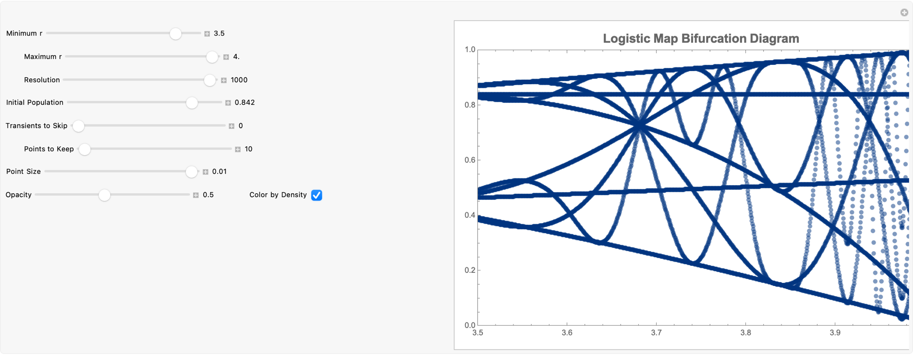
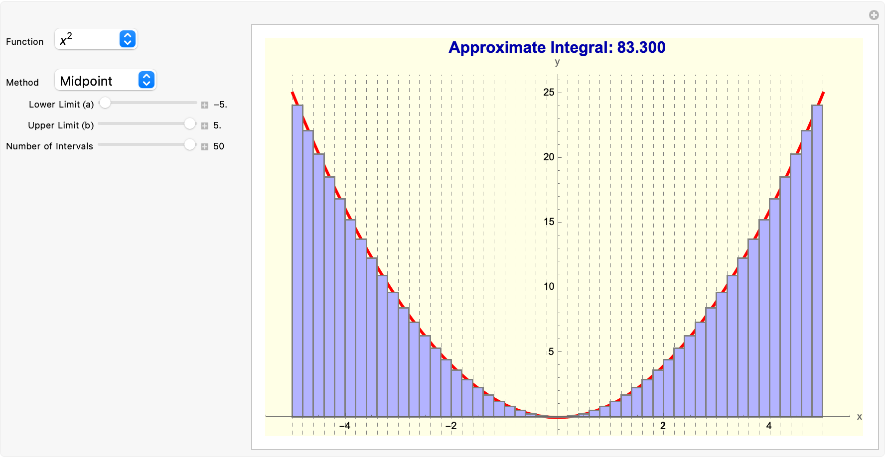
I used to think the thing to demonstrate is that all of these demonstrations revolve primarily around the concept of Riemann sums and the area between curves integration, you name it. But now, from the logistic map's chaos perspective to standard Riemann sum visualizers, it turns out that students can additionally and always pick "Left", "Right", "Midpoint", "Trapezoidal" (a method to set intervals n) and, watch as the approximated area converges still to the "Exact" integral value.

ClearAll["Global*"];
Manipulate[
 Module[{f, data, rVal, transient, orbit}, 
  f[r_, x_] := r  x  (1 - x);
  data = Table[rVal = rMin + (rMax - rMin)*i/res;
    transient = Nest[f[rVal, #] &, x0, skip];
    orbit = NestList[f[rVal, #] &, transient, keep - 1];
    Table[{rVal, orbit[[j]]}, {j, 1, keep}], {i, 0, res}];
  ListPlot[Flatten[data, 1], PlotRange -> {{rMin, rMax}, {0, 1}}, 
   PlotStyle -> {PointSize[pointSize], Opacity[opacity], 
     If[colorDensity, Hue[0.6, 1, 0.5], Black]}, 
   AspectRatio -> 1/GoldenRatio, AxesLabel -> {"r", "x"}, 
   Frame -> True, 
   PlotLabel -> Style["Logistic Map Bifurcation Diagram", Bold, 16], 
   ImageSize -> 600]], 
 Row[{Control[{{rMin, 2.5, "Minimum r"}, 0, 4, 
     Appearance -> "Labeled"}], Spacer[20], 
   Control[{{rMax, 4, "Maximum r"}, rMin, 4, 
     Appearance -> "Labeled"}], Spacer[20], 
   Control[{{res, 300, "Resolution"}, 50, 1000, 50, 
     Appearance -> "Labeled"}]}], 
 Row[{Control[{{x0, 0.5, "Initial Population"}, 0, 1, 
     Appearance -> "Labeled"}], Spacer[20], 
   Control[{{skip, 100, "Transients to Skip"}, 0, 500, 10, 
     Appearance -> "Labeled"}], Spacer[20], 
   Control[{{keep, 100, "Points to Keep"}, 10, 200, 10, 
     Appearance -> "Labeled"}]}], 
 Row[{Control[{{pointSize, 0.001, "Point Size"}, 0.001, 0.01, 0.001, 
     Appearance -> "Labeled"}], Spacer[20], 
   Control[{{opacity, 0.5, "Opacity"}, 0.1, 1, 0.1, 
     Appearance -> "Labeled"}], Spacer[20], 
   Control[{{colorDensity, True, "Color by Density"}, {False, 
      True}}]}], 
 TrackedSymbols :> {rMin, rMax, res, x0, skip, keep, pointSize, 
   opacity, colorDensity}, Paneled -> True, ControlPlacement -> Left, 
 SynchronousUpdating -> False]

These concepts, the Riemann sums and derivatives, make it more and more obvious that when these derivatives come to life, each student grasps the material better also and develops a mindset that values efficiency and innovation--qualities that make it easier for researchers who perhaps might just want to get a McFlurry and some fries or however they like to reclaim and balance the day-to-day responsibilities of teaching and administrative duties with the desire for pedagogical, excellence. The fraction of their time that academics actually get to spend doing research and learning and thinking and so on..is surprisingly small. A lot of our computational paradigm is about just giving me the answer or seeing immediate numeric results. That's exactly the motivation behind Wolfram Demonstrations. The point there is just "Give me the answer", not "Point me to web pages". Because, once the approach gets below a threshold of difficulty, then you actually do it. We can weave in the pedagogical value of Wolfram Demonstrations in teaching IBDP Calculus: computational tools can bring us from classroom learning to genuine research innovation and back. As @Hasan Khan faithfully noted in his post, abstract concepts will become more accessible, in the classroom. They can do more than just flail and clarify the basics--they can also serve as a springboard for innovative research and smoothen out our use of time to be more efficient.

Manipulate[Module[{f, steps, cobweb}, f[x_] := r  x  (1 - x);
  steps = NestList[f, x0, n];
  cobweb = 
   Line[Join[{{x0, x0}}, 
     Flatten[Table[{{steps[[i]], steps[[i + 1]]}, {steps[[i + 1]], 
         steps[[i + 1]]}}, {i, 1, n}], 1]]];
  Plot[{f[x], x}, {x, 0, 1}, PlotRange -> {{0, 1}, {0, 1}}, 
   Epilog -> {Red, cobweb, PointSize[0.02], 
     Point[Transpose[{steps, steps}]]}, 
   PlotLabel -> Style[StringForm["Cobweb Diagram (r = `)", r], 16], 
   ImageSize -> 500, Frame -> True, FrameLabel -> {"x", "f(x)"}, 
   GridLines -> Automatic, GridLinesStyle -> LightGray]], {{r, 2.5, 
   "Parameter r"}, 0, 4, 
  Appearance -> "Labeled"}, {{x0, 0.5, "Initial x"}, 0, 1, 
  Appearance -> "Labeled"}, {{n, 5, "Iterations"}, 1, 20, 1, 
  Appearance -> "Labeled"}, TrackedSymbols :> {r, x0, n}, 
 Alignment -> Center, ControlPlacement -> Left]

Sparking innovation is seeing all these plots which often ignite student curiosity far beyond the standard IBDP Calculus curriculum. If you find that wrinkle in time in which you can do genuine exploration, that's something to be cherished. For instance let's say you're cooling down some coffee and you want to bridge the gap between standard calculus topics and real exploratory excitement some of which we derive from these illustrations. You turn on the air conditioner and are quite ecstatic to find the Wolfram Demonstrations, and the code blocks that circulate above..educators and students alike are able to manipulate models whether they're just checking in to sprinkle some entailment cones or whether they're exploring "what if" scenarios--an approach that is invaluable in both academic research and practical problem solving. While traditional academic roles can often limit the time available for the web-like structure of computability & complexity, tools like Wolfram Demonstrations, these code blocks that circulate, provide a balanced type of approach that, instead of focusing on administrative tasks, allows these tasks to fail and spend more time on creative problem solving, which just shows how this ultimately worked out to nurture an environment where researchers can flourish.

High-school students who can see an integral's numeric approximation update in real time are more likely to take some time to experiment and truly understand e.g. how subinterval size, affects their Riemann sum. All these code blocks tell the story of a remarkable approach in-line with the overarching message of the [WSS22] Teaching IBDP Calculus with Wolfram Demonstration efficiency in exploring abstract concepts, which is how educators can spend less time on busywork and more on prompting students' questions. If one were to say, pick a creative iteration and look at the code blocks, they're easy to adapt so a teacher can relax and craft tangents, integrals, or logistic bifurcations their way.

ClearAll["Global*"];
Manipulate[
 Module[{f, F, aVal}, f[x_] := 4   Sin[5   x]   Exp[-x/5] + 3;
  F[x_] = Integrate[f[t], {t, 0, x}];
  aVal = a;
  Column[{Row[{Show[
       Plot[f[x], {x, 0, 20}, PlotStyle -> {Purple, Thickness[0.005]},
         PlotRange -> {{0, 20}, {-1, 7}}, 
        AxesLabel -> {Style["x", Italic, 14], 
          Style["f(x)", Italic, 14]}, ImageSize -> 350, 
        PlotRangePadding -> Scaled[0.1], ImagePadding -> 20], 
       Plot[f[x], {x, 0, aVal}, Filling -> Axis, 
        PlotStyle -> {Purple, Thickness[0.005]}, 
        PlotRange -> {{0, 20}, {-1, 7}}, 
        PlotRangePadding -> Scaled[0.1], ImagePadding -> 20], 
       Graphics[{{Orange, Dashed, Thickness[0.002], 
          Line[{{aVal, -1}, {aVal, 7}}]}}]], Spacer[20], 
      Show[Plot[F[x], {x, 0, 20}, 
        PlotStyle -> {Orange, Thickness[0.005]}, PlotRange -> All, 
        AxesLabel -> {Style["x", Italic, 14], 
          Style["F(x)", Italic, 14]}, ImageSize -> 350, 
        PlotRangePadding -> Scaled[0.1], ImagePadding -> 20, 
        Epilog -> {{Orange, PointSize[0.02], 
           Point[{aVal, F[aVal]}]}}]]}, Alignment -> Center], 
    Spacer[10], 
    Row[{Style["F(a) = \[Integral] f(x) dx = ", 16, Italic, 
       Darker@Orange], 
      Style[NumberForm[F[aVal], {5, 2}], 16, Bold, Darker@Orange]}, 
     Alignment -> Center]}, Alignment -> Center]], {{a, 10, 
   "Upper limit (a)"}, 0.01, 20, 0.1, 
  Appearance -> {"Labeled", "Open"}, ControlPlacement -> Top}, 
 TrackedSymbols :> {a}, Paneled -> True, FrameMargins -> None, 
 SaveDefinitions -> True]

The principle of expository clarity righteously vindicates our approach to teaching. Instead of drawing the same Riemann diagram by hand some arbitrary number of times, we can apply the same principle of expository clarity and thereby let the code handle it arbitrarily, then focus on students' critical thinking about integral convergence. For example, students see how $F(a) = \int_0^a f(x) \,dx$ accumulates area under f(x) from 0 up to a. When they watch the dashed vertical line move, shading the region between the curve and the x-axis, simultaneously a second plot shows the integral's running total. We describe small changes to input producing big & instantly visible results in modern computational tools. This is precisely the advantage of turning up the noise on manipulation. Students can shift the upper limit (a) slider from 0 to 20 and watch the integral's value build in real-time.

Manipulate[
 Module[{f, xvals, verticalSteps, horizontalSteps, cobwebPoints}, 
  f[x_] := r  x  (1 - x);
  xvals = NestList[f, x0, n];
  verticalSteps = 
   Table[{xvals[[i]], xvals[[i + 1]]}, {i, 1, Length[xvals] - 1}];
  horizontalSteps = 
   Table[{xvals[[i + 1]], xvals[[i + 1]]}, {i, 1, 
     Length[xvals] - 1}];
  cobwebPoints = 
   Join[{{x0, 0}}, 
    Flatten[Transpose[{verticalSteps, horizontalSteps}], 1]];
  Show[Plot[{f[x], x}, {x, 0, 1}, 
    PlotStyle -> {Directive[Blue, Thickness[0.005]], 
      Directive[Gray, Dashed]}, AxesLabel -> {"x", "f(x)"}, 
    PlotRange -> {{0, 1}, {0, 1}}, ImageSize -> 500, 
    Epilog -> {Red, PointSize[0.02], Point[{x0, 0}]}], 
   Graphics[{Thickness[0.002], Red, Line[cobwebPoints]}]]], {{r, 3.0, 
   "Parameter r"}, 2.5, 4.0, 
  Appearance -> "Labeled"}, {{x0, 0.2, "Initial x₀"}, 0.0, 1.0, 
  Appearance -> "Labeled"}, {{n, 50, "Iterations"}, 1, 100, 1, 
  Appearance -> "Labeled"}, TrackedSymbols :> {r, x0, n}]

Shift from "area under a curve" to "accumulation". In these code blocks I unify the notion of integrals as sums. The demonstration colors each rectangle left-endpoint vs. midpoint vs. right-endpoint differentially and displays, the numeric difference from the actual integral..it's our star-gazing approach that explains how we underscore efficiency and clear exposition--these are two crucial components in turning raw ideas into results--teachers can make the concept of integration vivid without static snapshots or half-drawn rectangles on the whiteboard. If you want to do research, you have to be efficient enough. Push other things aside; you can spend more time on creative problem-solving.

Clear["Global*"];
p1 = -x^3 + x^2 + 12   x - 2;
p2 = Sin[x];
p3 = Cos[x];
xmin = -6;
xmax = 6;
dx = (xmax - xmin)/5;
Manipulate[
 With[{f = gr, df = D[gr, x]}, 
  Grid[{{Plot[f, {x, xmin, xmax}, 
      PlotRange -> {{xmin - 0.5, xmax + 0.5}, 
        If[gr === p1, {-150, 150}, {-1.5, 1.5}]}, 
      AxesLabel -> {"x", "f(x)"}, ImageSize -> 400, 
      PlotStyle -> {Black, Thickness[0.005]}, 
      Epilog -> {{Blue, Thickness[0.005], 
         Line[{{xi - dx, (f /. x -> xi) - dx   (df /. x -> xi)}, {xi +
              dx, (f /. x -> xi) + dx   (df /. x -> xi)}}]}, {Red, 
         Thickness[0.005], 
         Line[{{xi, f /. x -> xi}, {xi + h, 
            f /. x -> xi + h}}]}, {Red, PointSize[0.02], 
         Point[{{xi, f /. x -> xi}, {xi + h, 
            f /. x -> xi + h}}]}, {Black, PointSize[0.02], 
         Point[{xi, f /. x -> xi}]}, 
        Inset[Style[
          Row[{"Secant slope: ", 
            NumberForm[(f /. x -> xi + h - f /. x -> xi)/h, {5, 3}]}],
           12, Bold, Red], Scaled[{0.15, 0.9}]], 
        Inset[Style[
          Row[{"Derivative: ", NumberForm[df /. x -> xi, {5, 3}]}], 
          12, Bold, Blue], Scaled[{0.15, 0.8}]]}], 
     Plot[(f /. x -> xi + hh - f /. x -> xi)/hh, {hh, -1, 1}, 
      Exclusions -> hh == 0, PlotRange -> {Automatic, {-50, 50}}, 
      AxesLabel -> {"h", "Difference Quotient"}, ImageSize -> 400, 
      PlotStyle -> {Black, Thickness[0.005]}, 
      Epilog -> {{Dashed, Blue, 
         Line[{{-1, df /. x -> xi}, {1, df /. x -> xi}}]}, {Red, 
         PointSize[0.02], 
         Point[{h, (f /. x -> xi + h - f /. x -> xi)/h}]}, 
        Inset[Style["Slope as h \[RightArrow] 0", 12, Bold, Blue], 
         Scaled[{0.5, 0.9}]]}]}}]], {{gr, p1, 
   "Function"}, {p1 -> "Cubic: -x³ +x² +12x -2", p2 -> "Sine: sin(x)",
    p3 -> "Cosine: cos(x)"}, 
  ControlType -> PopupMenu}, {{xi, 0, Subscript["x", 0]}, xmin, xmax, 
  0.1, Appearance -> "Labeled"}, {{h, 0.5, "h"}, -1, 1, 0.01, 
  Appearance -> "Labeled"}, TrackedSymbols :> {gr, xi, h}]

Revisit the Epsilon-Delta with a cubic and a parametric Riemann sum. We also have these tangent lines and integrals that explain the trigonometric variations on visualizing tangents & derivatives & integrals and general limit concepts. These are prime International Baccalaureate Diploma Programme Calculus materials. Each focuses on a slightly different slice of "Why derivative?" or "Why Riemann sums?".

ClearAll["Global*"];
Manipulate[
 Module[{f, dx, samples, rectangles, sum, xmin, xmax}, 
  f = Function[x, Evaluate[selectedFunction]];
  dx = (b - a)/n;
  xmin = a;
  xmax = b;
  sum = Which[method == "Left", Sum[f[a + i*dx]*dx, {i, 0, n - 1}], 
    method == "Right", Sum[f[a + (i + 1)*dx]*dx, {i, 0, n - 1}], 
    method == "Midpoint", Sum[f[a + (i + 0.5)*dx]*dx, {i, 0, n - 1}], 
    method == "Trapezoidal", 
    Sum[(f[a + i*dx] + f[a + (i + 1)*dx])/2*dx, {i, 0, n - 1}]];
  rectangles = 
   Which[method == "Left", 
    Table[{EdgeForm[Gray], Lighter[Blue, 0.7], 
      Rectangle[{a + i*dx, 0}, {a + (i + 1)*dx, f[a + i*dx]}]}, {i, 0,
       n - 1}], method == "Right", 
    Table[{EdgeForm[Gray], Lighter[Blue, 0.7], 
      Rectangle[{a + i*dx, 0}, {a + (i + 1)*dx, 
        f[a + (i + 1)*dx]}]}, {i, 0, n - 1}], method == "Midpoint", 
    Table[{EdgeForm[Gray], Lighter[Blue, 0.7], 
      Rectangle[{a + i*dx, 0}, {a + (i + 1)*dx, 
        f[a + (i + 0.5)*dx]}]}, {i, 0, n - 1}], 
    method == "Trapezoidal", 
    Table[{EdgeForm[Gray], Lighter[Blue, 0.7], 
      Polygon[{{a + i*dx, 0}, {a + (i + 1)*dx, 0}, {a + (i + 1)*dx, 
         f[a + (i + 1)*dx]}, {a + i*dx, f[a + i*dx]}}]}, {i, 0, 
      n - 1}]];
  Show[Plot[f[x], {x, xmin, xmax}, 
    PlotStyle -> {Red, Thickness[0.005]}, 
    PlotRange -> {{xmin - 0.5, xmax + 0.5}, Automatic}, 
    AxesLabel -> {"x", "y"}, ImageSize -> 600], 
   Graphics[{rectangles}], 
   PlotLabel -> 
    Style[Row[{"Approximate Integral: ", 
       NumberForm[sum, {\[Infinity], 3}]}], 16, Bold, Darker@Blue], 
   GridLines -> {Table[a + i*dx, {i, 0, n}], None}, 
   GridLinesStyle -> Directive[Gray, Dashed], 
   Background -> Lighter[Yellow, 0.9]]], 
 Grid[{{"Function", 
    PopupMenu[
     Dynamic[selectedFunction], {x^2 -> TraditionalForm[x^2], 
      Sin[x] -> TraditionalForm[Sin[x]], 
      Cos[x] -> TraditionalForm[Cos[x]], 
      Exp[x] -> TraditionalForm[e^x], 
      Log[x + 1] -> TraditionalForm[ln   (x + 1)]}, 
     ImageSize -> All]}, {"Method", 
    PopupMenu[
     Dynamic[method], {"Left", "Right", "Midpoint", "Trapezoidal"}]}},
   Alignment -> Left, 
  Spacings -> {1, 2}], {{a, 0, "Lower Limit (a)"}, -5, 5, 0.1, 
  Appearance -> "Labeled", 
  ImageSize -> Small}, {{b, 2, "Upper Limit (b)"}, -5, 5, 0.1, 
  Appearance -> "Labeled", 
  ImageSize -> Small}, {{n, 5, "Number of Intervals"}, 1, 50, 1, 
  Appearance -> "Labeled", ImageSize -> Small}, 
 ControlPlacement -> Left, 
 TrackedSymbols :> {selectedFunction, a, b, n, method}, 
 SynchronousUpdating -> False]

That's why we repeatedly stress that a big part of mastering a skill--be it advanced math or entrepreneurship--is about writing code or building small demos to test out ideas rapidly. Teachers can do the same, whether it's modeling an asteroid or finding that niche where you get to do research & learning. Hopefully contributing good things to the world that's a niche you know, to be cherished. These interactive code blocks give teachers a "niche" where exploration can happen swiftly, be repeated, and help students see the bigger picture behind the micro mechanics of calculus. Diagrams, I like the ambiance plus converse of https://demonstrations.wolfram.com/TheCoffeeCoolingProblem/#more to be quite honest if you see them you'll understand what it means to calculate the area of a rectangle, which is unilaterally reminiscent of the logistic map bifurcation diagrams.

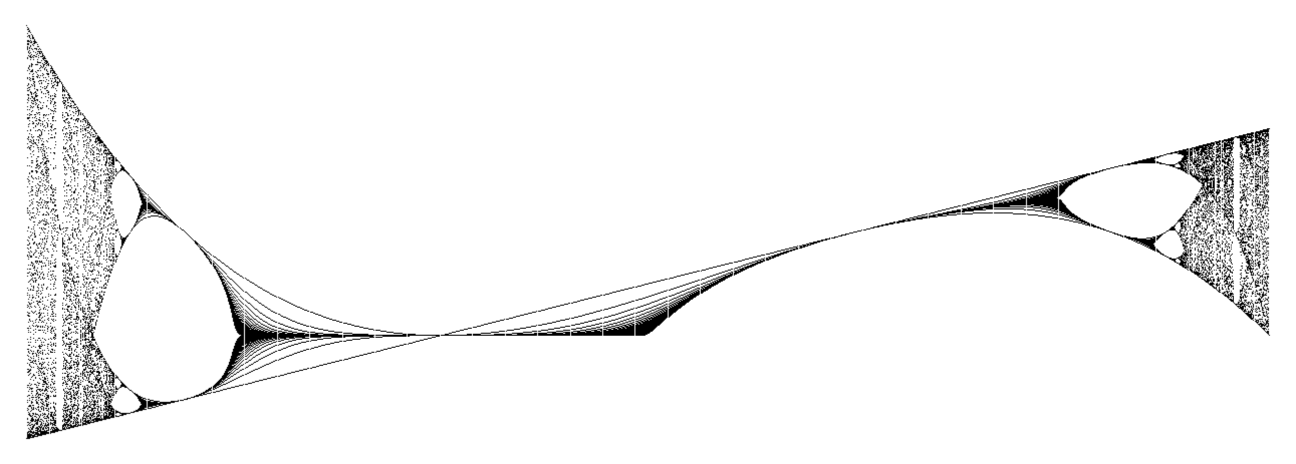
acc = {};
Subscript[f, r_][x_] := (1 - x) x r;
Do[{Do[orbit[r][n] = {r, 
     NestList[Subscript[f, r], 0.25 r, 100][[n]]}, {n, 100}];
  acc = Join[acc, Table[orbit[r][n], {n, 100}]]}, {r, -2, 4, .005}]
Graphics[{PointSize[.0001], Point[acc]}]

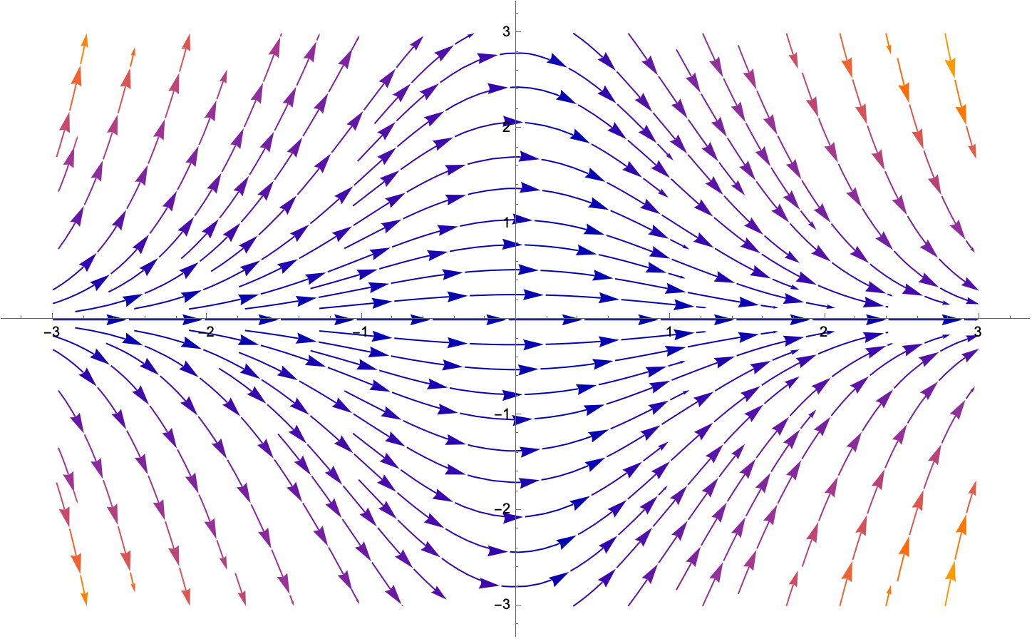
The thicker the cream, the smaller the thermal conductivity. Are you sure you want to make a coffee cooler? Wouldn't it be cool to see this but for the linear amplification, the heat coefficient of pure coffee and coffee (with cream) such as dT/dt = h⋅(0 - T), h = 0.4, instantaneously with a small amount of coffee and a massive amount of cream.

It reminds me of pouring the cream in the coffee immediately. The cream's already at room temperature right?

f[h_, T_] = 
 h (0 - T); StreamPlot[{1, f[h, T]}, {h, -3, 3}, {T, -3, 3}, 
 Frame -> False, Axes -> True, AspectRatio -> 1/GoldenRatio]

If you put it in it's like a buffer against the rate of heat loss, but butter and cream affect the coffee's temperature differently; butter's thermal conductivity is much less than that of water, and creams would be better mixed into the hot coffee so butter's warmth-keeping mechanism is totally different from that of cream's.