But it's really the multi-headed approach that unfurls interconnected multiway states, as multiple active cells evolve concurrently. This approach honestly increases the complexity of branchial graphs and gives fertile ground for analyzing computational irreducibility and complexity. For instance. Let's say we want to multi-headed automatonedly initialize the computation of the branchial complexity metrics, such as state growth and graph connectivity measures. The proper analogy for this would be of course "ordering the Italian beef"; more heads or rules are introduced, scaling complexity. I guess so, branchial graphs for multi-headed automata composed of 3 to 5 active cells exhibit increasing connectivity, suggesting a combinatorial explosion in possible states. Utilizing Mathematica's built-in graph functions, one can quantify these changes.
ClearAll["Global`*"];
stripMetadata[expr_] := If[Head[expr] === Rule, Last[expr], expr];
getMAStateGraphics3D[rule_, state_, time_] :=
  Module[{stateData = ToExpression[stripMetadata[state]]},
   ListPointPlot3D[
    Table[{i, stateData[[i]], time}, {i, Length[stateData]}],
    PlotStyle -> {Directive[PointSize[0.03],
       ColorFunction -> (Hue[#3/(time + 1)] &),
       ColorFunctionScaling -> False]},
    PlotRange -> {{1, Length[stateData]}, {0, 1}, {0, time + 1}},
    AxesLabel -> {"Cell", "State", "Time"}, BoxRatios -> {1, 1, 1},
    ImageSize -> 400,
    PlotLabel ->
     Style["3D Multiway State", Bold, 14, FontFamily -> "Arial"]]];
stateRenderingFunction3D[rule_] :=
  Inset[getMAStateGraphics3D[rule, #2, #3], #1, Center, #4] &;
stateEvolutionFunction3D[state_String, rules_List] :=
  ToString /@ (ResourceFunction["MobileAutomaton"][ToExpression[#],
        ToExpression[state], 1][[-1]] & /@ rules);
MultiwayMobileAutomaton3D[rules_List, initialConditions_List,
   stepCount_Integer, rest___] :=
  ResourceFunction["MultiwaySystem"][
   Association[
    "StateEvolutionFunction" -> (stateEvolutionFunction3D[#1,
        rules] &), "StateEquivalenceFunction" -> SameQ,
    "StateEventFunction" -> (# &),
    "EventDecompositionFunction" -> Function[{a, b, c}, None],
    "EventApplicationFunction" -> Function[{a, b, c}, None],
    "SystemType" -> "MobileAutomaton",
    "EventSelectionFunction" -> Identity],
   ToString /@ initialConditions, stepCount, rest,
   "StateRenderingFunction" -> stateRenderingFunction3D[First[rules]],
    "EventRenderingFunction" -> Function[{a, b, c}, None]];
MobileAutomatonPlot2D[evolution_, opts : OptionsPattern[ArrayPlot]] :=
   Module[{dataArray, height}, dataArray = evolution[[All, 1]];
   height = Length[evolution];
   Show[ArrayPlot[dataArray, FilterRules[{opts}, Options[ArrayPlot]],
     ColorRules -> {0 -> Red, 1 -> Blue}, PlotRange -> All,
     Frame -> True, FrameTicks -> None, ImageSize -> 400],
    Graphics@
     MapIndexed[
      With[{row = #2[[1]], heads = #1},
        Table[Disk[{pos - 0.5, (height - row) + 0.5}, 0.25], {pos,
          heads}]] &, evolution[[All, 2]]]]];
firstRuleChoices = <|"Growth" -> {275, 999}, "Spiral" -> {90, 150},
   "Chaotic" -> {30, 60}|>;
secondRuleChoices = <|"Wave" -> {81, 384}, "Stripe" -> {22, 45},
   "Fractal" -> {110, 158}|>;
graphLayouts = {"LayeredDigraphEmbedding" -> "Layered",
   "SpringElectricalEmbedding" -> "Spring",
   "CircularEmbedding" -> "Circular", "RadialEmbedding" -> "Radial",
   "BalloonEmbedding" -> "Balloon"};
DynamicModule[{firstRuleChoice = "Growth", secondRuleChoice = "Wave",
  firstRuleManual = {275, 999}, secondRuleManual = {81, 384},
  tapeLength = 15, headPos = 8, steps = 3, highlightDepth = 2,
  vertexSize = 0.5, layoutChoice = "LayeredDigraphEmbedding",
  allRules = {}, showRulesText = "{{275,999},{81,384}}",
  initTapeText = "", addRuleIndex = 0},
 Panel[Style[
   Column[{Row[{Style["Primary Rule (1A\[Dash]1B): ", Bold, 12,
        FontFamily -> "Arial"],
       PopupMenu[Dynamic[firstRuleChoice, (firstRuleChoice = #;

           If[KeyExistsQ[firstRuleChoices, #],
            firstRuleManual = firstRuleChoices[#], Null];) &],
        Append[Keys[firstRuleChoices], "Manual Input..."],
        ImageSize -> 120], Spacer[10],
       Dynamic[If[firstRuleChoice === "Manual Input...",
         InputField[Dynamic[firstRuleManual], FieldSize -> {8, 1},
          BaseStyle -> {FontFamily -> "Courier"}], ""],
        TrackedSymbols :> {firstRuleChoice}], Spacer[20],
       Style["Secondary Rule (2A\[Dash]2B): ", Bold, 12,
        FontFamily -> "Arial"],
       PopupMenu[Dynamic[secondRuleChoice, (secondRuleChoice = #;

           If[KeyExistsQ[secondRuleChoices, #],
            secondRuleManual = secondRuleChoices[#], Null];) &],
        Append[Keys[secondRuleChoices], "Manual Input..."],
        ImageSize -> 120], Spacer[10],
       Dynamic[If[secondRuleChoice === "Manual Input...",
         InputField[Dynamic[secondRuleManual], FieldSize -> {8, 1},
          BaseStyle -> {FontFamily -> "Courier"}], ""],
        TrackedSymbols :> {secondRuleChoice}]}], Spacer[10],
     Row[{Style["Tape (Array) Length:", Bold, 12,
        FontFamily -> "Arial"],
       Slider[Dynamic[tapeLength], {5, 35, 1}, ImageSize -> 200],
       Dynamic[tapeLength], Spacer[20],
       Style["Active Cell Head Position:", Bold, 12,
        FontFamily -> "Arial"],
       Slider[Dynamic[headPos], {Floor[tapeLength/2],
         1 + (Floor[tapeLength/2]), Floor[tapeLength/2]},
        ImageSize -> 200], Dynamic[headPos]}], Spacer[10],
     Row[{Style["Evolution Exploration Steps:", Bold, 12,
        FontFamily -> "Arial"],
       Slider[Dynamic[steps], {1, 6, 1}, ImageSize -> 200],
       Dynamic[steps], Spacer[20],
       Style["Highlight Depth:", Bold, 12, FontFamily -> "Arial"],
       Slider[Dynamic[highlightDepth], {0, 6, 1}, ImageSize -> 200],
       Dynamic[highlightDepth]}], Spacer[10],
     Row[{Style["Vertex Node Size:", Bold, 12, FontFamily -> "Arial"],
        Slider[Dynamic[vertexSize], {0.1, 2, 0.1}, ImageSize -> 200],
       Dynamic[vertexSize], Spacer[20],
       Style["Graph Layout:", Bold, 12, FontFamily -> "Arial"],
       PopupMenu[Dynamic[layoutChoice], graphLayouts,
        ImageSize -> 150]}], Spacer[15],
     Row[{Button["Add Rule", (addRuleIndex++;

         AppendTo[
          allRules, {RandomInteger[{0, 999}],
           RandomInteger[{0, 999}]}];),
        BaseStyle -> {"GenericButton", Bold, FontFamily -> "Arial"},
        ImageSize -> {80, 30}], Spacer[10],
       Button["Reset", (allRules = {};
         addRuleIndex = 0;
         firstRuleChoice = "Growth";
         secondRuleChoice = "Wave";
         firstRuleManual = {275, 999};
         secondRuleManual = {81, 384};
         tapeLength = 15;
         headPos = 8;
         steps = 3;
         highlightDepth = 2;
         vertexSize = 0.5;
         layoutChoice = "LayeredDigraphEmbedding";
         showRulesText = "{{275,999},{81,384}}";
         initTapeText = "";),
        BaseStyle -> {"GenericButton", Bold, FontFamily -> "Arial"},
        ImageSize -> {80, 30}], Spacer[20],
       Column[{Style["All Rules (text area):", Bold, 12,
          FontFamily -> "Arial"],
         InputField[Dynamic[showRulesText], FieldSize -> {40, 2},
          BaseStyle -> {FontFamily -> "Courier"},
          FieldHint -> "e.g. {{275,999},{81,384}}"],
         Style["(Paste multiple rules here to override.)", Italic, 10,
           FontFamily -> "Arial"]}]}], Spacer[10],
     Row[{Column[{Style["Initial State (Alternate):", Bold, 12,
          FontFamily -> "Arial"],
         Style["(Enter e.g. {0,0,1,0,1}, overriding the \
\[OpenCurlyQuote]Tape Length\[CloseCurlyQuote] slider.)", Italic, 10,
          FontFamily -> "Arial"],
         InputField[Dynamic[initTapeText], FieldSize -> {40, 2},
          BaseStyle -> {FontFamily -> "Courier"}]}]}], Spacer[10],
     Dynamic[Module[{firstRuleUsed, secondRuleUsed, mergedRules,
        initialTape, initialConfig, mg3D, graphLayoutOption},
       firstRuleUsed =
        If[KeyExistsQ[firstRuleChoices, firstRuleChoice],
         firstRuleChoices[firstRuleChoice],
         If[firstRuleChoice === "Manual Input...",
          firstRuleManual, {275, 999}]];
       secondRuleUsed =
        If[KeyExistsQ[secondRuleChoices, secondRuleChoice],
         secondRuleChoices[secondRuleChoice],
         If[secondRuleChoice === "Manual Input...",
          secondRuleManual, {81, 384}]];
       mergedRules =
        Quiet[Check[
          ToExpression[
           showRulesText], {{firstRuleUsed, secondRuleUsed}}]];
       If[! ListQ[mergedRules],
        mergedRules = {{firstRuleUsed, secondRuleUsed}}];
       If[Length[allRules] > 0,
        mergedRules = Join[mergedRules, allRules]];
       initialTape =
        Quiet[Check[ToExpression[initTapeText],
          ConstantArray[0, tapeLength]]];
       If[! ListQ[initialTape],
        initialTape = ConstantArray[0, tapeLength]];
       headPos = Min[headPos, Length[initialTape]];
       If[headPos < 1, headPos = 1];
       initialConfig = {{initialTape, headPos}};
       graphLayoutOption =
        Switch[layoutChoice, "LayeredDigraphEmbedding",
         "LayeredDigraphEmbedding", "SpringElectricalEmbedding",
         "SpringElectricalEmbedding", "CircularEmbedding",
         "CircularEmbedding", "RadialEmbedding", "RadialEmbedding",
         "BalloonEmbedding", "BalloonEmbedding", _,
         "LayeredDigraphEmbedding"];
       mg3D =
        MultiwayMobileAutomaton3D[mergedRules, initialConfig, steps,
         "StatesGraphStructure", VertexSize -> vertexSize,
         GraphLayout -> graphLayoutOption];
       With[{vFirst = VertexList[mg3D][[1]],
         outcomp =
          VertexOutComponent[mg3D, VertexList[mg3D][[1]],
           highlightDepth]},
        HighlightGraph[
         mg3D, {Style[vFirst, Red], Style[outcomp, Yellow]},
         Background -> Transparent,
         VertexStyle ->
          Directive[EdgeForm[{Thick, Hue[0.6, 1, 0.8]}],
           Specularity[White, 50]],
         EdgeStyle -> Directive[Opacity[0.6], Hue[0.6, 0.5, 0.8]],
         PlotLabel ->
          Style["3D Multiway Mobile Automaton", Bold, 16,
           FontFamily -> "Arial"], ImageSize -> Large]]],
      TrackedSymbols :> {firstRuleChoice, secondRuleChoice,
        firstRuleManual, secondRuleManual, tapeLength, headPos, steps,
         highlightDepth, vertexSize, layoutChoice, showRulesText,
        allRules, initTapeText}], Spacer[20],
     Dynamic[Module[{rule1x, evolutionData},
       rule1x =
        If[KeyExistsQ[firstRuleChoices, firstRuleChoice],
         firstRuleChoices[firstRuleChoice],
         If[firstRuleChoice === "Manual Input...",
          firstRuleManual, {275, 999}]];
       Module[{thisTape},
        thisTape =
         Quiet[Check[ToExpression[initTapeText],
           ConstantArray[0, tapeLength]]];
        If[! ListQ[thisTape], thisTape = ConstantArray[0, tapeLength]];
        evolutionData =
         ResourceFunction["MobileAutomaton"][
          rule1x, {thisTape, headPos}, steps];
        Column[{Style["Automaton Evolution (2D) Using First Rule",
           Bold, 14, FontFamily -> "Arial"],
          MobileAutomatonPlot2D[evolutionData, Mesh -> True]}]]],
      TrackedSymbols :> {firstRuleChoice, firstRuleManual, tapeLength,
         headPos, steps, initTapeText}]}]]]]
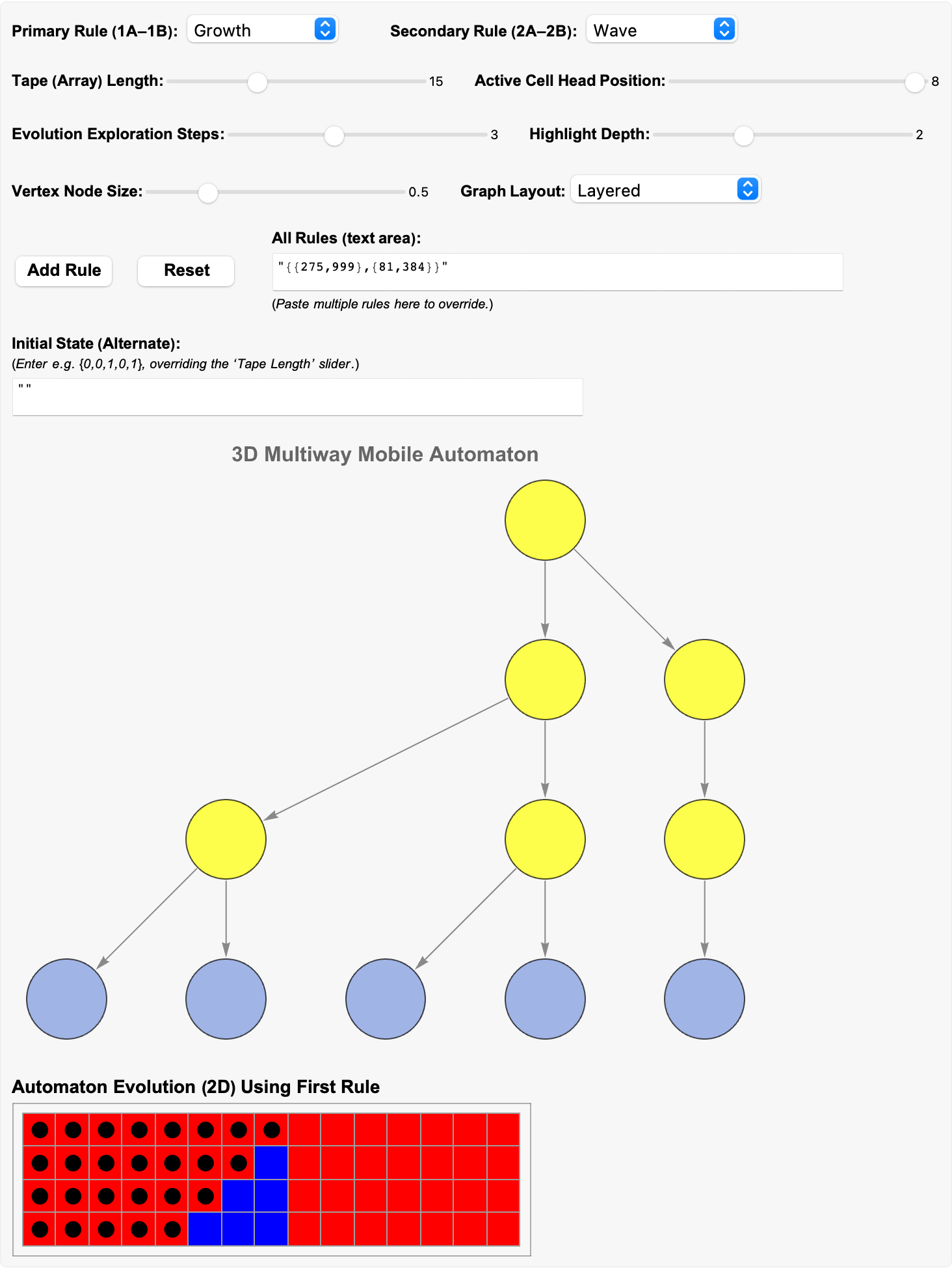
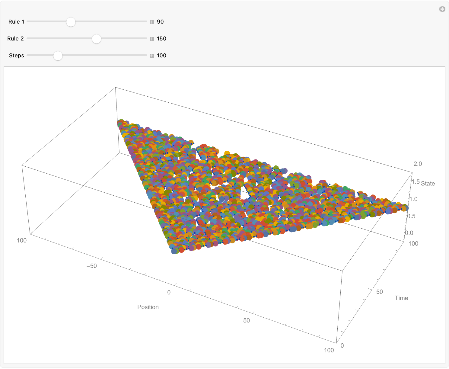
Theoretical research, into parallels between computational systems and physical phenomena, such as phase transitions and causal structures flourescently portraying relativistic light cones. Because after all, "no one has to know" the, information propagation speed. No one is going to care if we used probabilistic methods or we say we handled increased computational demands. Because, we test multiway mobile automata as models for concurrent or distributed computation. Look at this. I have no idea why the 275 to 999, the 90 to 150, the 30 to 60 play out this way but they do so, here's the color gradient based on "time-step progression"--the evolution history of states within a multiway system. The scariest thing of all is how these complexity analyses are enabled, by advanced Mathematica functionalities.


That was the rule set 275 to rule 999, rule 81 to rule 384.


That was the rule 90 to 150, 22 to 45.


We did it, we already cycled through the rules..30 to 60, 110 to 158..the componentized approach tells us that, all these embeddings look the same if you look at them closely you'll see, that the Layered Digraph is identical to the Radial is identical and so on and so forth. I think that better understanding the rule icons using MobileAutomatonRulePlot, is something that graphically explains how each rule operates. And this will..for the rule pair {275, 999}, aid in the comprehension of their effects on the automaton's evolution. Because now we can define a set of preset rules and allow users to select them via a dropdown menu.
ClearAll["Global`*"];
stripMetadata[expr_] := If[Head[expr] === Rule, Last[expr], expr];
getMAStateGraphics3D[rule_, state_] :=
Framed[Style[
ResourceFunction["MobileAutomatonPlot"][
ResourceFunction["MobileAutomaton"][rule, state, 0],
ColorRules -> {0 -> White}, Mesh -> True], Hue[0.62, 1, 0.48]],
Background -> Directive[Opacity[0.2], Hue[0.62, 0.45, 0.87]],
FrameMargins -> {{2, 2}, {0, 0}}, RoundingRadius -> 0,
FrameStyle -> Directive[Opacity[0.5], Hue[0.62, 0.52, 0.82]]];
stateRenderingFunction3D[rule_] :=
Inset[getMAStateGraphics3D[rule,
ToExpression[stripMetadata[#2]]], #1, Center, #3] &;
statesEvolutionFunction3D[state_String, rules_List] :=
ToString /@ (ResourceFunction["MobileAutomaton"][ToExpression[#1],
ToExpression[state], 1][[-1]] & /@ rules);
MultiwayMobileAutomaton3D[rules_List, initialConds_List,
steps_Integer, rest___] :=
ResourceFunction["MultiwaySystem"][<|
"StateEvolutionFunction" -> (statesEvolutionFunction3D[#1,
rules] &), "StateEquivalenceFunction" -> SameQ,
"StateEventFunction" -> (# &),
"EventDecompositionFunction" -> Function[{a, b, c}, None],
"EventApplicationFunction" -> Function[{a, b, c}, None],
"SystemType" -> "MobileAutomaton",
"EventSelectionFunction" -> Identity|>, ToString /@ initialConds,
steps, rest,
"StateRenderingFunction" -> stateRenderingFunction3D[First[rules]],
"EventRenderingFunction" -> Function[{a, b, c}, None]];
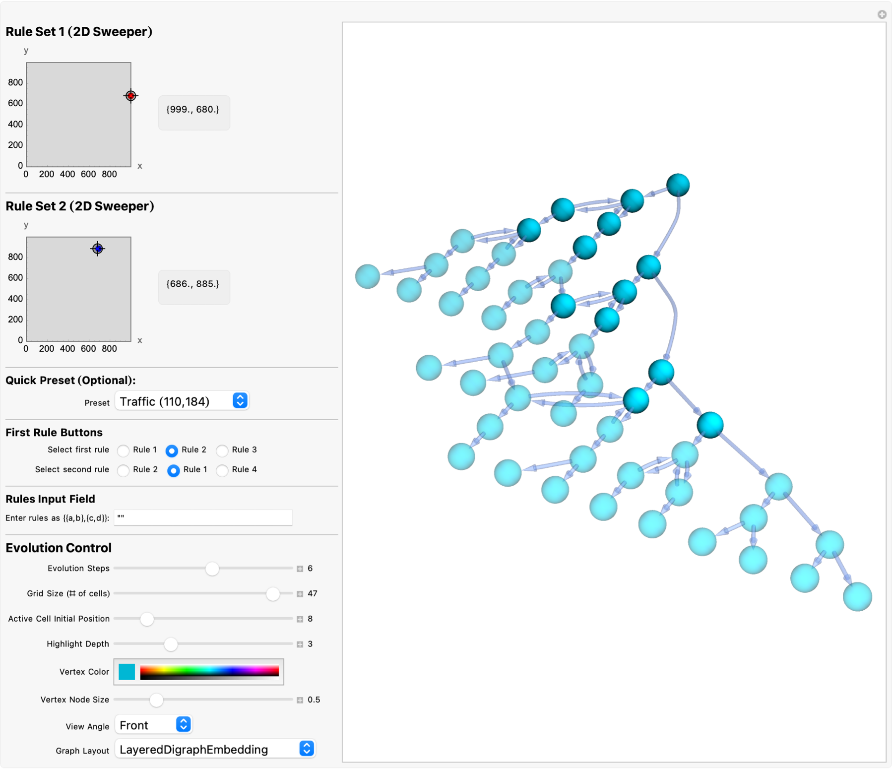
DynamicModule[{rule1 = {275, 999}, rule2 = {81, 384}},
Manipulate[
Module[{allRules, initialState, g, topVertex, toHighlight},
allRules = {Round[rule1], Round[rule2]};
Quiet[
If[rulesInputField =!= "",
With[{parsed = ToExpression[rulesInputField]},
If[ListQ[parsed] && AllTrue[parsed, ListQ],
allRules = parsed]]]];
initialState = {ConstantArray[0, gridSize], activeCell};
g = MultiwayMobileAutomaton3D[allRules, {initialState}, steps,
"StatesGraphStructure", VertexSize -> vertexSize];
topVertex = If[VertexList[g] =!= {}, VertexList[g][[1]], None];
toHighlight =
If[topVertex =!= None,
VertexOutComponent[g, topVertex, highlightDepth], {}];
HighlightGraph[
Graph3D[g, VertexStyle -> Directive[theColor],
EdgeStyle -> Directive[Opacity[0.5], Hue[0.62, 0.52, 0.82]],
ImageSize -> Large, Boxed -> False, RotationAction -> "Clip",
PlotRangePadding -> 0.5, ViewPoint -> viewAngle,
GraphLayout -> graphLayoutChoice], toHighlight,
GraphHighlightStyle -> "DehighlightFade"]], Delimiter,
Style["Rule Set 1 (2D Sweeper)", Bold, 14],
Row[{LocatorPane[Dynamic[rule1],
Graphics[{LightGray, EdgeForm[Gray],
Rectangle[{0, 0}, {999, 999}], Red, PointSize[Large],
Point[Dynamic[rule1]]}, Axes -> True, AxesLabel -> {"x", "y"},
PlotRange -> {{0, 999}, {0, 999}}, ImageSize -> 150]],
Spacer[10], Dynamic@Panel[rule1, ImageSize -> {80, 40}]},
Alignment -> Center], Delimiter,
Style["Rule Set 2 (2D Sweeper)", Bold, 14],
Row[{LocatorPane[Dynamic[rule2],
Graphics[{LightGray, EdgeForm[Gray],
Rectangle[{0, 0}, {999, 999}], Blue, PointSize[Large],
Point[Dynamic[rule2]]}, Axes -> True, AxesLabel -> {"x", "y"},
PlotRange -> {{0, 999}, {0, 999}}, ImageSize -> 150]],
Spacer[10], Dynamic@Panel[rule2, ImageSize -> {80, 40}]},
Alignment -> Center], Delimiter,
Style["Quick Preset (Optional):", Bold,
12], {{presetChoice, None, "Preset"}, {None -> "None",
"Elementary 30/90" -> "Elementary (30,90)",
"Traffic 110/184" -> "Traffic (110,184)"},
ControlType -> PopupMenu}, Delimiter,
Style["First Rule Buttons", Bold,
12], {{firstRuleChoice, "Rule 1", "Select first rule"}, {"Rule 1",
"Rule 2", "Rule 3"},
ControlType -> RadioButtonBar}, {{secondRuleChoice, "Rule 2",
"Select second rule"}, {"Rule 2", "Rule 1", "Rule 4"},
ControlType -> RadioButtonBar}, Delimiter,
Style["Rules Input Field", Bold,
12], {{rulesInputField, "", "Enter rules as {{a,b},{c,d}}:"},
String, FieldSize -> {24, 1}}, Delimiter,
Style["Evolution Control", Bold,
14], {{steps, 5, "Evolution Steps"}, 1, 10, 1,
Appearance -> "Labeled"}, {{gridSize, 15,
"Grid Size (# of cells)"}, 5, 50, 1,
Appearance -> "Labeled"}, {{activeCell, 8,
"Active Cell Initial Position"}, 1, Dynamic[gridSize], 1,
Appearance -> "Labeled"}, {{highlightDepth, 2, "Highlight Depth"},
0, 10, 1,
Appearance -> "Labeled"}, {{theColor, Hue[0.62, 1, 0.48],
"Vertex Color"},
ColorSlider}, {{vertexSize, 0.5, "Vertex Node Size"}, 0.1, 2, 0.1,
Appearance -> "Labeled"}, {{viewAngle, {1.3, -2.4, 2.0},
"View Angle"}, {{1.3, -2.4, 2.0} -> "Standard", {0, 0, 3} ->
"Top", {3, 0, 1} -> "Side", {0, -3, 1} -> "Front"},
ControlType -> PopupMenu}, {{graphLayoutChoice,
"LayeredDigraphEmbedding",
"Graph Layout"}, {"LayeredDigraphEmbedding",
"SpringRadialCircularEmbedding"}, ControlType -> PopupMenu},
TrackedSymbols :> {rule1, rule2, presetChoice, firstRuleChoice,
secondRuleChoice, rulesInputField, steps, gridSize, activeCell,
highlightDepth, theColor, vertexSize, viewAngle,
graphLayoutChoice}, Paneled -> True, FrameMargins -> 10
]
]
To analyze the complexity and connectivity of the resulting graphs, we compute metrics such as the average degree & clustering coefficient & graph diameter. I think the application of graphMetrics yields statistics about the structure and complexity of the automaton's evolution, in the observatory perspective of the rotational animations and controls, which differentiate the viewpoint of the 3-Dimensional graph comprehensively, and exploratorially structure our exploration. And it's almost time to..look go for some additional signs of life in the Ruliad. So far we've been finding a few MCASteps, proceeding with an initial set of Ruliological rules and constructs and, it's a bit of a jumpscare cause whenever Mathematica crashes I just uninstall it. So there, you may have to uninstall Mathematica and reinstall it just to fulfill our quest of being Ruliologically able to run all the latest code. The important thing remember is that at least my Mathematica installation, when it crashes it does so so quietly. You can always restart the kernel it's not like RStudio, which makes this incessant beep when it (R) crashes. Remember, each crash brings us closer to understanding the profound structures that come out of simple rules, and the Ruliad offers a boundless frontier for discovery. Of course yes, working with such complex systems can sometimes lead to software instability. Restarting the kernel or reinstalling the software may be necessary to continue your journey into and out of the depths, of computational complexity. As we continue our exploration into the Ruliad, the vast space of all possible computational rules, these tools and matrices and metrics become exponential. They not only help us identify signs of complex behavior but they have every credential, they also guide us in selecting and evaluating the consistency of new rule sets.
Furthermore, the use of rotational animations and interactive controls in our 3-Dimensional visualizations allows for a comprehensive exploration of the graph's structure from multiple perspectives. This interstellar viewpoint builds down our understanding of the automaton's behavior and the delicate patterns that span time and space. By trying to apply the graphMetrics function to our graphs, we obtain these statistics, which shed light on the structural complexity and evolution of the automaton. And that may not even be worth explaining how the graph diameter, is referentially the longest shortest path between "any" two nodes in the graph, reflecting the graph's reachability in all its scintillated nodes and folds, to form the clustering coefficient; the measure of the formation of tightly knit groups, which is indicative as always of the presence of the local clusters within the graph. But so what if I always need to explain stuff (Version 14 this time had me installing astrology, then it had me installing calculus etc.)..the Wolfram Community thinks it's just so cool. I'll tell you, the complexity and connectivity of the graphs had my Mathematica going, from multiway mobile automata, and that is how we got the computation of several metrics not to mention the mean number of connections, per node, offering the graph some connectivity that is worth noting. Because if you're an academic, you might think you get to spend all day every day kind of learning, doing research, but you don't. It's really the story of my life, I've managed to make my life efficient enough that I can do this, even though I do have a day job of running a tech company.
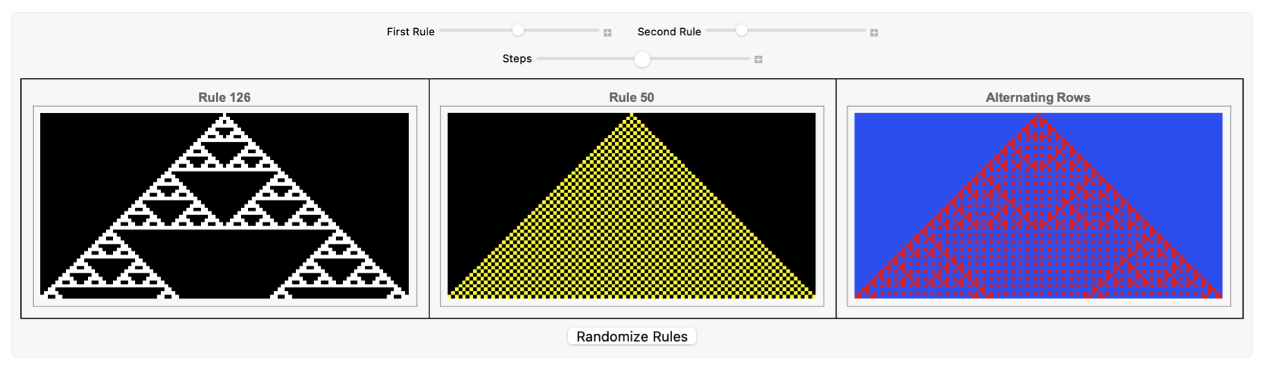
DynamicModule[{rule1 = 30, rule2 = 90, steps = 50, size = 101,
  initial, ca1, ca2, combined}, initial = ConstantArray[0, size];
 initial[[Ceiling[size/2]]] = 1;
 Panel[Column[{Row[{Control[{{rule1, 30, "First Rule"}, 0, 255, 1,
        ImageSize -> 150}], Spacer[20],
      Control[{{rule2, 90, "Second Rule"}, 0, 255, 1,
        ImageSize -> 150}]}, Alignment -> Center],
    Control[{{steps, 50, "Steps"}, 1, 100, 1, ImageSize -> Medium}],
    Dynamic[ca1 = CellularAutomaton[{rule1, 2}, initial, steps];
     ca2 = CellularAutomaton[{rule2, 2}, initial, steps];
     combined =
      MapIndexed[If[OddQ[First[#2]], #1, ca2[[First[#2]]]] &, ca1];
     Grid[{{ArrayPlot[ca1, ColorFunction -> "SunsetColors",
         ImageSize -> Medium,
         PlotLabel -> Style["Rule " <> ToString[rule1], Bold]],
        ArrayPlot[ca2, ColorFunction -> "AvocadoColors",
         ImageSize -> Medium,
         PlotLabel -> Style["Rule " <> ToString[rule2], Bold]],
        ArrayPlot[combined, ColorFunction -> "TemperatureMap",
         ImageSize -> Medium,
         PlotLabel -> Style["Alternating Rows", Bold]]}},
      Spacings -> {2, 2}, Frame -> All, Alignment -> Center]],
    Button["Randomize Rules", {rule1 = RandomInteger[{0, 255}],
      rule2 = RandomInteger[{0, 255}]}, ImageSize -> Medium]},
   Alignment -> Center], ImageMargins -> 10]]
The best trick is to find a niche in the world where the things you want to do are somehow valued. I know it isn't the most masculine thing but, we have to excuse it because, remember there's the whole entire section of the Wolfram Community that focuses on Raspberry Pi. Looking for answers..most people don't do very well in the sensory-deprivation-tank situation--they need something practical and stimulating alongside pure research. That's why if you don't understand what you're writing about, your readers won't stand a chance. There'll always be unforeseen loopholes; computational irreducibility guarantees that that three simple laws of robotics are that, LLM-generated writing is kind of flat--I call that a routine explanation, but not for things that haven't been explained before; don't just defer to self-proclaimed experts--ask lots of questions, drill down, and trust that there's an underlying logic you can learn. And earn, believe in yourself, build something you want to use that has a much higher chance of success than building something you don't care about (at all) but think the world will. So yea, when search and the web came along, you discovered questions you'd never thought to ask--once the barrier "goes down", you actually use the tool.
ClearAll[MultiwayMobileAutomaton, stripMetadata, getMAStateGraphics,
  stateRenderingFunction, stateEvolutionFunction];
stripMetadata[expression_] :=
  If[Head[expression] === Rule, Last[expression], expression];
getMAStateGraphics[rule_, state_] :=
  Framed[Style[
    ResourceFunction["MobileAutomatonPlot"][
     ResourceFunction["MobileAutomaton"][rule, state, 0],
     ColorRules -> {0 -> White}, Mesh -> True,
     MeshStyle -> Directive[Gray, Dashed]], FontFamily -> "Helvetica",
     FontSize -> 14, FontWeight -> "Medium"],
   Background ->
    Directive[Opacity[0.15], Lighter[Hue[0.62, 0.45, 0.87], 0.3]],
   FrameMargins -> 5, RoundingRadius -> 10,
   FrameStyle ->
    Directive[Opacity[0.7], Lighter[Hue[0.62, 0.52, 0.82], 0.3],
     Thick]];
stateRenderingFunction[rule_] :=
  Inset[getMAStateGraphics[rule, ToExpression[stripMetadata[#2]]], #1,
     Center, #3] &;
stateEvolutionFunction[state_String, rules_List] :=
  ToString /@ (ResourceFunction["MobileAutomaton"][ToExpression[#1],
        ToExpression[state], 1][[-1]] & /@ rules);
MultiwayMobileAutomaton[rules_List, initialConditions_List,
   stepCount_Integer, rest___] :=
  ResourceFunction["MultiwaySystem"][
   Association[
    "StateEvolutionFunction" -> (stateEvolutionFunction[#1, rules] &),
     "StateEquivalenceFunction" -> SameQ,
    "StateEventFunction" -> Identity,
    "EventDecompositionFunction" -> (Null &),
    "EventApplicationFunction" -> (Null &),
    "SystemType" -> "MobileAutomaton",
    "EventSelectionFunction" -> Identity],
   ToString /@ initialConditions, stepCount, rest,
   "StateRenderingFunction" -> stateRenderingFunction[First[rules]],
   "EventRenderingFunction" -> (Null &)];
Manipulate[
 Module[{rules = {{rule1a, rule1b}, {rule2a, rule2b}}, initial},
  initial = {{ConstantArray[0, size], pos}};
  MultiwayMobileAutomaton[rules, initial, steps,
   "StatesGraphStructure", GraphLayout -> layout,
   VertexSize -> vertexSize,
   EdgeStyle -> Directive[Opacity[0.3], GrayLevel[0.4]],
   VertexStyle ->
    Directive[EdgeForm[None], Lighter[Hue[0.6, 0.5, 0.8], 0.2]],
   ImageSize -> 600]], {{rule1a, 275, "First Rule Part 1"}, 1, 1000,
  1}, {{rule1b, 999, "First Rule Part 2"}, 1, 1000,
  1}, {{rule2a, 81, "Second Rule Part 1"}, 1, 1000,
  1}, {{rule2b, 384, "Second Rule Part 2"}, 1, 1000,
  1}, {{size, 35, "Initial Array Size"}, 10, 50, 1,
  Appearance -> "Labeled"}, {{pos, 17, "Active Cell Position"}, 1,
  size, 1, Appearance -> "Labeled"}, {{steps, 4, "Evolution Steps"},
  1, 8, 1, Appearance -> "Labeled"}, {{vertexSize, 0.8, "Node Size"},
  0.1, 2, 0.1,
  Appearance -> "Labeled"}, {{layout, "SpringEmbedding",
   "Graph Layout"}, {"SpringEmbedding", "LayeredDigraphEmbedding",
   "RadialEmbedding", "CircularEmbedding"}}, ControlPlacement -> Left,
  Paneled -> True, FrameMargins -> 10,
 TrackedSymbols :> {rule1a, rule1b, rule2a, rule2b, size, pos, steps,
   vertexSize, layout}]
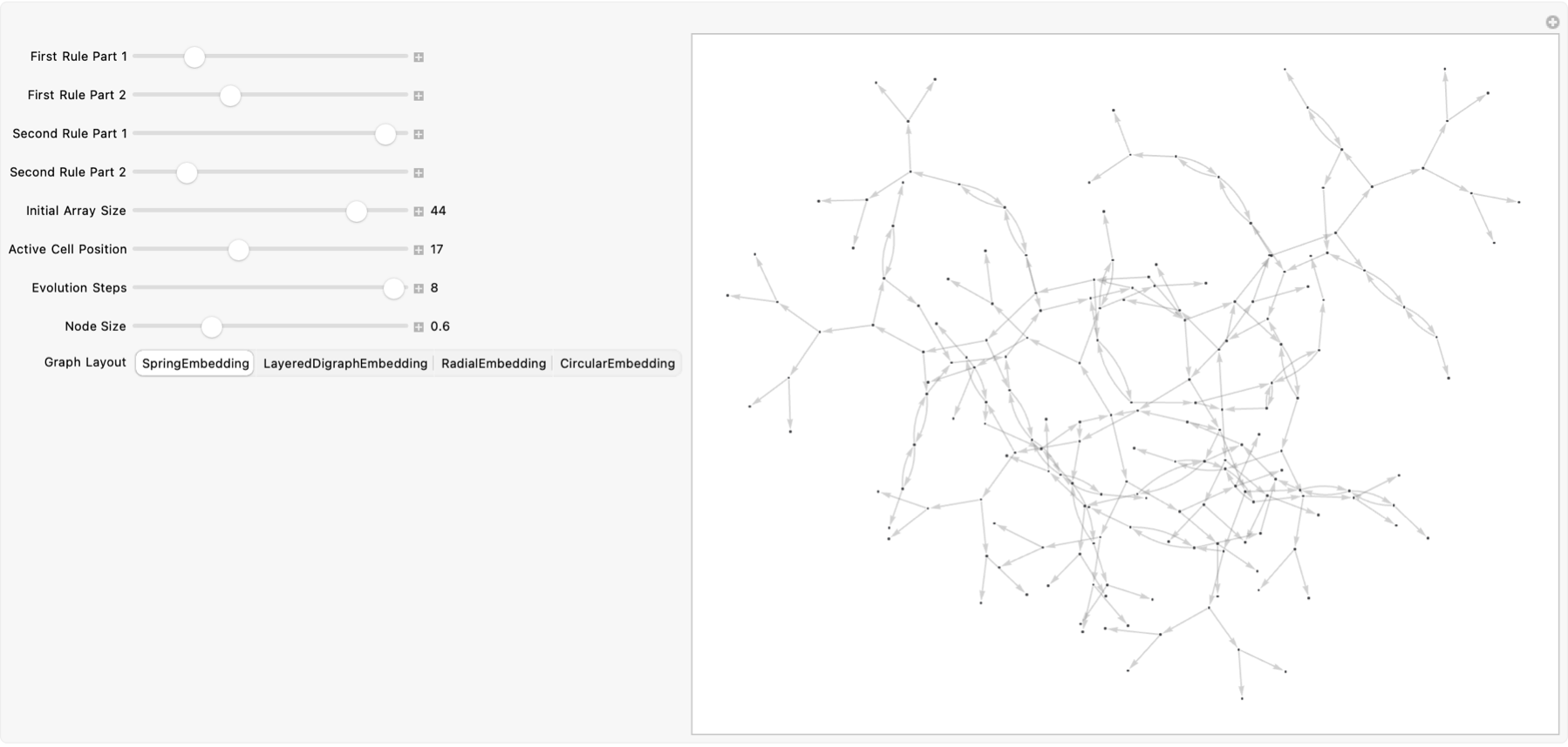
There's a lot of utility to stripping metadata; before any rendering or evolution can occur, you need to clean up the internal "Rule[...]" wrappers that Wolfram ResourceFunctions "sometimes" emit. In order to get a fully customizable multiway mobile automaton by combining two core ResourceFunctions--MobileAutomatonPlot for rendering individual automaton evolutions and MultiwaySystem for inter-branchial space--wrapped inside a Manipulate for branching, we first define utility routines to clean up metadata and render individual states, then stitch them together into a multiway network, and finally verify these sliders and menus for tweaking rule parameters, initial conditions, graph layout, as well as styling. When it comes to the documentation you'd better pick up that phone! Imagine running Mathematica on your cell phone..but anyway, make some little cuts--remove the rule wrappers and strip off the Rule[...] wrapper on the raw expression payload via Last if the head is Rule--and otherwise return the expression unchanged. And then you'd have a full complete subsequent functionality that always receives clean state data rather than rule objects. But we have to ask ourselves what is the, and this is just a helpful tip that we may have to do that because, with the getMAStateGraphics[rule_, state_] that calls to generate a grid-plot of a single mobile automaton evolution, then the newfangled Mathematica stateRenderingFunction insetting each state, the resulting graphics are then embedded into the multiway graph which has placed, each state-cell graphic at its vertex coordinates, permitting the multiway network to display each branch's evolution as a mini-plot.
MCAStep[{ru1_, ru2_}, {c_, b_, a_}] := {b, a,
  IntegerDigits[ru2, 2, 8][[
   8 - (#1 + 2 (#2 + 2 #3)) & @@ # & /@
    Transpose[{c, b,
      IntegerDigits[ru1, 2, 8][[
       8 - (RotateLeft[a] + 2 (a + 2 RotateRight[a]))]]}]]]}
Manipulate[
 Module[{evolution, points, initSize = 2*steps + 1},
  evolution =
   NestList[
    MCAStep[{ru1, ru2}, #] &, {Table[0, initSize], Table[0, initSize],
      CenterArray[{1}, initSize]}, steps];
  points =
   Flatten[Table[
     Position[evolution[[i, 3]], 1] /.
      pos_Integer :> {pos - initSize/2, i - 1, 1}, {i,
      Length[evolution]}], 1];
  ListPointPlot3D[points,
   PlotStyle -> {PointSize[0.015], Hue[0.6, 1, 0.7]},
   BoxRatios -> {2, 1, 0.5},
   PlotRange -> {{-initSize/2, initSize/2}, {0, steps}, All},
   AxesLabel -> {"Position", "Time", "State"}, ImageSize -> 700,
   AxesStyle -> Gray,
   PlotLabel ->
    Style[StringJoin["Rules ", ToString[ru1], " & ", ToString[ru2]],
     White, Bold, 16]]], {{ru1, 90, "Rule 1"}, 0, 255, 1,
  Appearance -> "Labeled"}, {{ru2, 150, "Rule 2"}, 0, 255, 1,
  Appearance -> "Labeled"}, {{steps, 100, "Steps"}, 10, 400, 10,
  Appearance -> "Labeled"}, ControlPlacement -> Top]
While this local vs. global multiway dichotomy exists, see "Local Multiway Systems" in the Wolfram Physics Project for more physics-oriented approaches, otherwise our local branching system, carries Mathematica expressions for which one can swap in ResourceFunction["MultiwayFunctionSystem"] for purely integer-based multiway functions, so cleaning metadata and parsing with Head/Last is a single-headed modularization of metadata stripping and per-state rendering as well as the instantaneous and rapid rearrangement of both the tree of states and the embedded 1-Dimensional automaton plots, customized by the following style--every node is a live plot instead of a plain label, making the system's behavior transparent visually and precomputing automaton slices and caching them becomes retrievable; for large sizes / steps, we want to avoid recalculating during every Manipulate refresh.
Manipulate[
 Module[{caRule1, caRule2, cellsRule1, cellsRule2,
   offset = steps + 1},
  caRule1 = CellularAutomaton[{rule1, 2}, {{1}, 0}, steps];
  caRule2 = CellularAutomaton[{rule2, 2}, {{1}, 0}, steps];
  cellsRule1 =
   Flatten[Table[
     If[caRule1[[i, j]] === 1, Cuboid[{j - offset, 0, i - 1}],
      Nothing], {i, 1, steps + 1}, {j, 1, 2*steps + 1}], 1];
  cellsRule2 =
   Flatten[Table[
     If[caRule2[[i, j]] === 1, Cuboid[{j - offset, 1, i - 1}],
      Nothing], {i, 1, steps + 1}, {j, 1, 2*steps + 1}], 1];
  Graphics3D[{{Red, Opacity[0.6], cellsRule1}, {Blue, Opacity[0.6],
     cellsRule2}}, Boxed -> True,
   PlotRange -> {{-offset, offset}, {0, 1}, {0, steps}},
   AxesLabel -> {"Cell Position", "Rule", "Time"},
   Ticks -> {Range[-offset, offset, 2], {0 -> "Rule 1",
      1 -> "Rule 2"}, Range[0, steps, 2]}, ImageSize -> 300,
   Lighting -> {{"Ambient", White}}, ViewPoint -> {3, 1, 1},
   BoxRatios -> {2, 0.1, 1}]],(*Controls*){{rule1, 30, "Rule 1"}, 0,
  255, 1, Appearance -> "Labeled"}, {{rule2, 90, "Rule 2"}, 0, 255, 1,
   Appearance -> "Labeled"}, {{steps, 20, "Steps"}, 1, 50, 1,
  Appearance -> "Labeled"}, ControlPlacement -> Left]
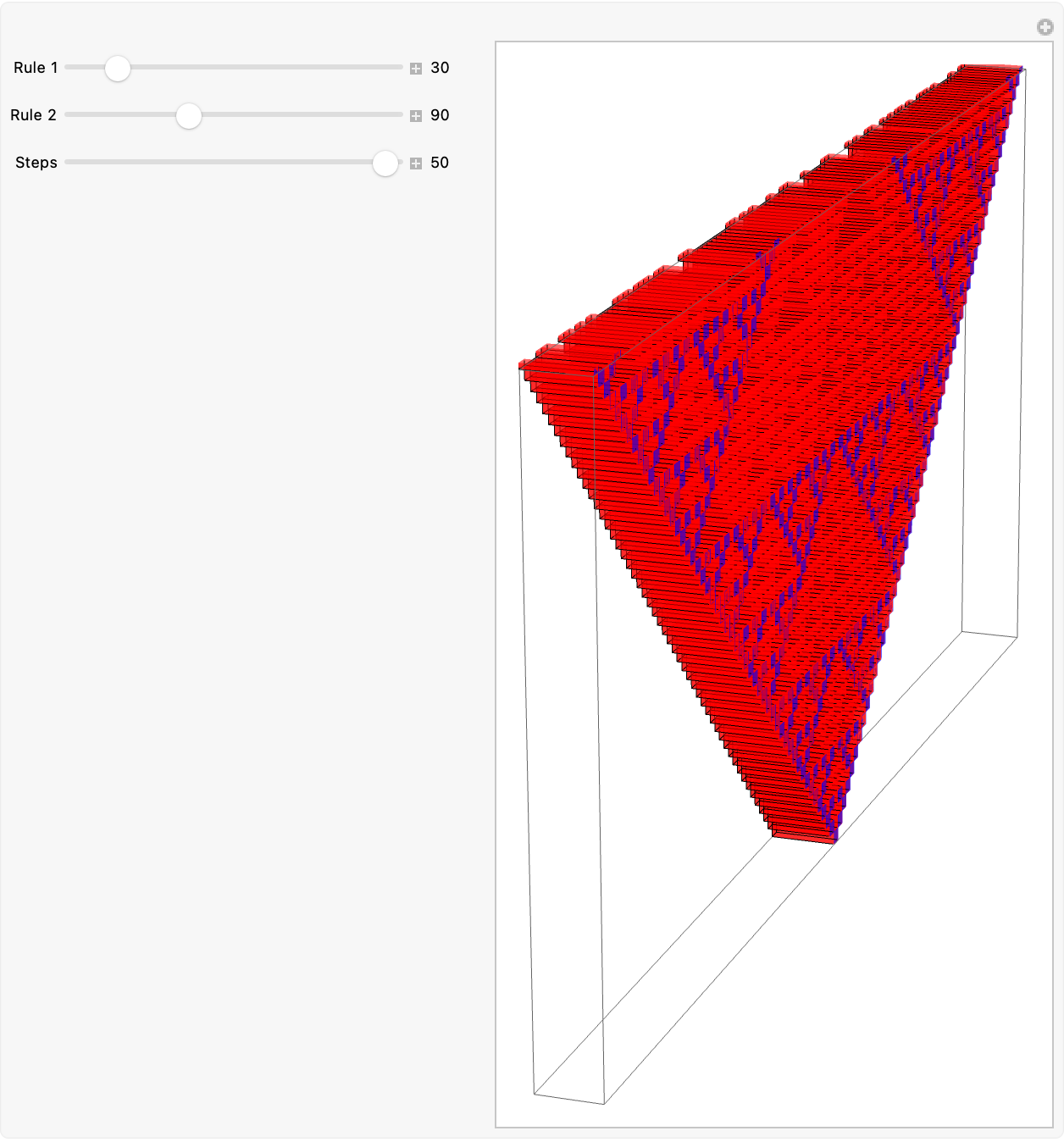
There's a whole new branch of software you should know out there that hasn't yet been explored. These multiway mobile automata, it's like living in a glass house, comparing two one-dimensional elementary cellular automata side-by-side, we compute the spatiotemporal evolution of two rules (rule1, rule2) for a user-specified number of steps, extract the "on" cells as 3-Dimensional cuboids, and color them red and blue at distinct Y-levels. Who does that? I can't possibly imagine how, also when I started thinking about designing some componentized Ruliological dimensions I realized there's so much more to it than we ever knew, different rules propagate information over time to obliquely separate the two layers uniformly without directional shadows. And there's tons of errors but what the heck, why not show each time step of the Elementary Cellular Automata with the given rule of course and range 1, since we know that a Cuboid we create at those coordinates where the cell value is 1, and confine Y to a two-level band at the center, of the spatial axis.
With[{ruleLeft = 40, ruleRight = 80,
  initialState = {1, 0, 1, 1, 0, 0, 1, 0, 1, 1, 0, 0},
  initialActive = 4, steps = 11, imgSize = 500},
 Module[{evol, states, activePos},
  evol = ResourceFunction["MobileAutomaton"][{ruleLeft,
     ruleRight}, {initialState, initialActive}, steps];
  states = evol[[All, 1]];
  activePos = evol[[All, 2]];
  Graphics3D[{Table[
     If[states[[t + 1, x]] == 1, {Hue[0.62, 1, 0.5, 0.7],
       Cuboid[{x - 1, t, 0}, {x, t + 1, 0.1}]}, {Opacity[0.1],
       Cuboid[{x - 1, t, 0}, {x, t + 1, 0.1}]}], {t, 0, steps}, {x, 1,
       Length[initialState]}], {Red,
     Table[Sphere[
       If[NumericQ[activePos[[t + 1]]], {activePos[[t + 1]] - 0.5, t,
         0.2}, {0, t, 0.2}], 0.2], {t, 0, steps}]}}, Boxed -> True,
   Axes -> True, AxesLabel -> {"Cell Position", "Step", ""},
   Lighting -> "Neutral",
   PlotRange -> {{0, Length[initialState]}, {0, steps}, {-1, 1}},
   ImageSize -> imgSize]]]
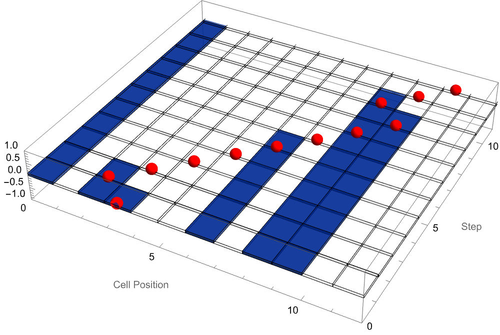
MobileAutomaton evolves a "mobile"..Turing-like automaton, returning {state,activePos} pairs, the community-published MobileAutomaton has the "characteristic' that data extraction via list operations can produce a layered 3-Dimensional plot showing both the binary cell patterns over time and the trajectory of the mobile (active) cell by combining Cuboid and Sphere and the rendering options for primitive geometrics, render spheres of specified radii at given points and add the Hue-Saturation-Brightness color directive scene, the Ruliad is huge. And I know it's a little far-fetched that's why I'm looking at the delicacies of raw state data which should, design good error-correcting code which is really sphere-packing in high dimensions, where each codeword is a center and errors are little spheres around it. Our brains run at a million times slower than transistors, yet remain far more energy-efficient and unbeatable at broad reasoning--showing there's still much to learn about molecular-scale computing. Which should ease us into the dimensional aspect of, regular polygons that and which are infinite in 2 dimensions but in 3 dimensions there are exactly five Platonic solids--and in 4 dimensions you get their higher-dimensional cousins like the 20-cell and tesseract. I'm pretty sure that's how you say it right? Tesseract?
MCAStep[{ru1_, ru2_}, {c_, b_, a_}] := {b, a,
   IntegerDigits[ru2, 2, 8][[
    8 - (#1 + 2 (#2 + 2 #3)) & @@ # & /@
     Transpose[{c, b,
       IntegerDigits[ru1, 2, 8][[
        8 - (RotateLeft[a] + 2 (a + 2 RotateRight[a]))]]}]]]};
Manipulate[
 Module[{evolution, data3D, size}, size = 2*initialSize + 1;
  evolution =
   NestList[
    MCAStep[{ru1, ru2}, #] &, {Table[0, size], Table[0, size],
     CenterArray[{1}, size]}, steps];
  data3D =
   Flatten[Table[
     If[evolution[[y, 3, x]] == 1,
      Cuboid[{x - initialSize - 1.5, y - 1.5,
        0}, {x - initialSize - 0.5, y - 0.5, 1}]], {y, 1,
      steps + 1}, {x, 1, size}], 1];
  Graphics3D[{EdgeForm[None], Hue[0.62, 1, 0.8], data3D},
   Lighting -> "Neutral",
   PlotRange -> {{-initialSize - 1, initialSize + 1}, All, {0, 1.2}},
   Boxed -> True, Axes -> True,
   AxesLabel -> {"Position", "Step", "State"}, ImageSize -> 800,
   RotationAction -> "Clip", ViewPoint -> {3, -1, 1.5}]], {{ru1, 164,
   "Primary Rule"}, 0, 255, 1,
  Appearance -> "Labeled"}, {{ru2, 61, "Secondary Rule"}, 0, 255, 1,
  Appearance -> "Labeled"}, {{initialSize, 20, "Initial Size"}, 5, 20,
   1, Appearance -> "Labeled"}, {{steps, 200, "Steps"}, 10, 200, 1,
  Appearance -> "Labeled"}, ControlPlacement -> Left]
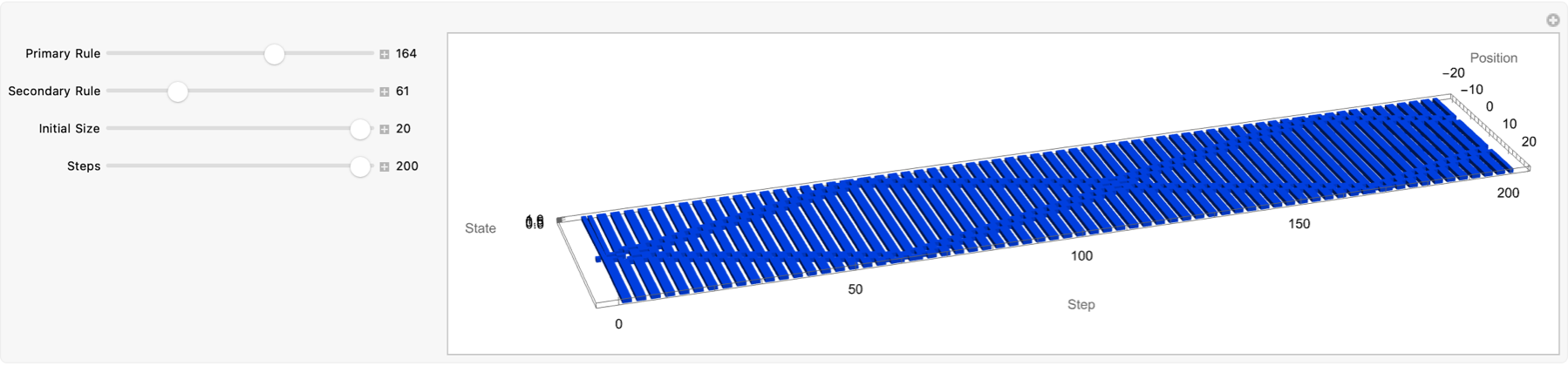
And I can't put a backslash at the "end of the file name", this Primary Secondary thing just underlies both holography and the uncertainty principle (think Fourier) signals and that's our signal, the very same math behind time-vs-frequency trade-offs in signals so for our purposes, and I know you've seen this MCAStep so many times. What it's doing is the "left" "center" and "right" neighborhoods are of equal length and have values of 0 / 1 at the current time step, so the two 8-bit rule numbers (each from 0 to 255) mean that the "intermediate" bits from ru1 convert ru1 into a fixed-length 8-bit list and, for each position in a compute a local index based on a 3-cell neighborhood of a itself and, index into the bits of ru1 (reversed by 8 - index) to get an "intermediate" 0 / 1 sequence of the same length, as a. To acquire the final state from ru2, form triples {c, b, intermediate} at each position, transpose into a list of length-3 vectors & compute, a standard Wolfram Cellular Automaton index i = c + 2 b + 4 intermediate and look up bit 8 - i in the 8-bit expansion of ru2. The result, is one new 0 / 1 list giving the updated "center" cell values. It was like a lightbulb went off in my head just for a moment. But that's why we're here. I don't want to say it but it's sort of a disembodied, truth that spatiotemporal, two-phase rule applications give so much better "dynamics" than a single Wolfram-style Cellular Automaton rule. Because the 3-dimensional space-time extrusion with Cuboid and Graphics3D neatly evolutionizes the coupling of two distinct rules which yields, complex behavior--and Mathematica, its flexible list and graphics primitives make such experiments concise yet interactive.
MCAStep[{ru1_, ru2_}, {c_, b_, a_}] := {b, a,
   IntegerDigits[ru2, 2,
     8][[8 - (#1 + 2  (#2 + 2  #3)) & @@ # & /@
      Transpose[{c, b,
        IntegerDigits[ru1, 2,
          8][[8 - (RotateLeft[a] +
             2  (a + 2  RotateRight[a]))]]}]]]};
DynamicModule[{ru1 = 90, ru2 = 150, t = 100},
 Panel[Column[{Row[{Control[{{ru1, 90, "Primary Rule"}, 0, 255, 1,
        Appearance -> "Labeled", ImageSize -> 300}], Spacer[20],
      Control[{{ru2, 150, "Secondary Rule"}, 0, 255, 1,
        Appearance -> "Labeled", ImageSize -> 300}]}],
    Row[{Control[{{t, 100, "Steps"}, 10, 500, 10,
        Appearance -> "Labeled", ImageSize -> 400}]}],
    Dynamic[Module[{raw, topGFX, topImg, reflImg, shimmered,
       amp = 4, \[Lambda] = 40, dims},
      raw = Last /@
        NestList[
         MCAStep[{ru1, ru2}, #] &, {ConstantArray[0, 2  t + 1],
          ConstantArray[0, 2  t + 1], CenterArray[{1}, 2  t + 1]},
         t];
      topGFX =
       ArrayPlot[raw, Frame -> False, PlotRange -> All,
        PlotRangePadding -> None, ImagePadding -> None,
        ImageSize -> {500, 250},
        ColorRules -> {0 -> Lighter[Gray, 0.923], 1 -> Black}];
      topImg = Rasterize[topGFX, ImageResolution -> 72];
      dims = ImageDimensions[topImg];
      reflImg =
       Rasterize[
        ArrayPlot[Reverse@Most[raw], Frame -> False, PlotRange -> All,
          PlotRangePadding -> None, ImagePadding -> None,
         ImageSize -> dims,
         ColorRules -> {0 -> Lighter[Gray, 0.923], 1 -> Black}],
        ImageResolution -> 72];
      shimmered =
       ImageTransformation[
        reflImg, (# + {amp*Sin[2*Pi*#[[2]]/\[Lambda]], 0} &),
        DataRange -> Full, Padding -> "Fixed"];
      ImageAssemble[{{topImg}, {shimmered}}, Background -> None]],
     TrackedSymbols :> {ru1, ru2, t}]}, Alignment -> Center],
  Background -> Lighter[Gray, 0.923]]]
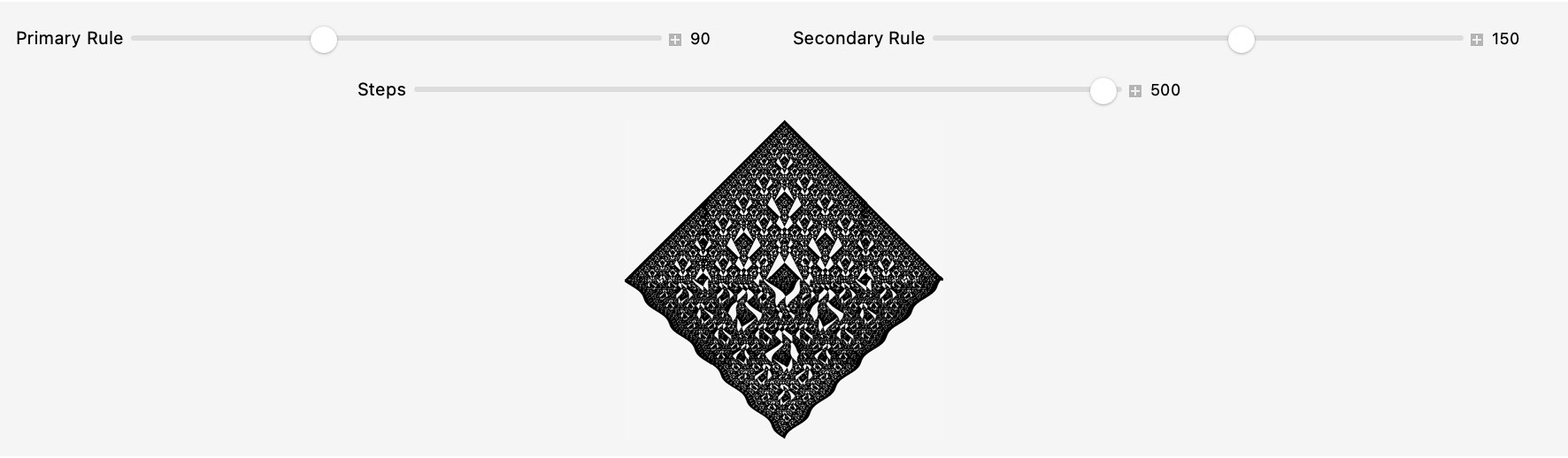
The thing to add with regard to these light waves is that they linearly add, which is great for interference-based tricks but problematic if you need the nonlinearity of a switch. There has to be a better way come on! Rasterization, wraps the raw binary evolution "in" ArrayPlot and then shifts sinusoidally, via ImageTransformation to create a shimmering reflection beneath and both, are combined with ImageAssemble. To be honest, what we'd really love is a decomposed neighborhood wherein {c, b, a} "look up" the left, center, and right bit-lists at the current step. Now I'd like to talk about how Last/@ extracts only the newly computed center-cell list from each triple but first, and they do say CenterArray[{1},2t+1] and the way it seeds a single "1" at the center of a zero-filled list of length 2t+1 is analogous, to cooking in the sense that our recipe is quality; no matter how you look at it, state 0 is not the same as state 1. That's why we need NestList[f,expr,n] to produce, states from step 0 through t by repeatedly applying MCAStep. I mean, of course there are many ways to stack the two images into one tall composite we're all adults--but the ImageAssemble[{ {img1}, {img2} }] constructs this composite original over its shimmering reflection. That's why I had to do this it's like making a casserole; you flip the copy vertically Reverse@Most[raw] which becomes the reflection, so each output pixel at {x,y} samples input at f[{x,y}] so it's okay because a sine-based horizontal shift is what creates the ripple, which becomes the projection of the notebook graphic into a fixed-resolution image via Rasterize[graphics,...]. And, so let's say you picked the rule numbers (0-255) and evolution depth (t up to 500). That's typically not within our interactive session, so let's persist with the following thought--so you put your car in IDLE and you've already converted ru1 into the 8-bit binary form with zero-left-padding and you've computed the index for each position in a, the index i = a_{l} + 2a + 4a_{r} via RotateLeft and RotateRight to access its 3-cell neighborhood. We can lookup the bit 8-i in the binary digits of ru1 to form an intermediate list like you said. But then we can lookup a secondary rule out of our back, position transposed "onto" a list of 3-dimensional vectors, computed for triples {c, b, intermediate} at each position, the j = c + 2 b + 4 intermediate and "index into" the 8-bit expansion of ru2, thus we have shifted gears and now, the function yields {b, a, newState} effectively, sliding the window forward by one cell each step. Mathematica gives us the superpower, to fly it's like Danny Phantom. It's really Mathematica that uniquely integrates the symbolic rule definition so it's not just the list processing it's also the built-in graphics / image functions..I would personally like to see some more MCAStep integrated into the documentation but that's not going to happen that fast. I just thought it was amazing how intermediate bits can be wrapped in sliders for two rule numbers and a step count, which evolves our single-seed initial condition for t iterations. That's basic binary evolution.
MCAStep[{ru1_, ru2_}, {c_, b_, a_}] := {b, a,
  IntegerDigits[ru2, 2, 8][[
   8 - (#1 + 2 (#2 + 2 #3)) & @@ # & /@
    Transpose[{c, b,
      IntegerDigits[ru1, 2, 8][[
       8 - (RotateLeft[a] + 2 (a + 2 RotateRight[a]))]]}]]]}
With[{t = 500},
 ArrayPlot[
  Last /@ NestList[
    MCAStep[{90, 150}, #] &, {Table[0, 2 t + 1], Table[0, 2 t + 1],
     CenterArray[{1}, 2 t + 1]}, t]]]
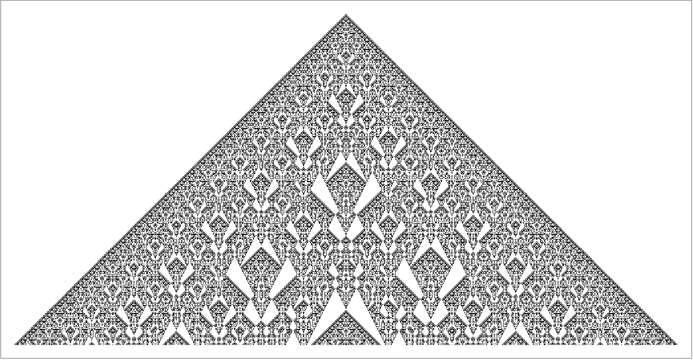
It is something where the sort of whole computational irreducibility story is quite relevant. I tend to think that eventually we will have more of an overarching theory of biology than we have "right now". Biology has been rather allergic to theory "just" because a lot of simple theories don't work in biology. Biology has this sort of meta feature that usually if you try and explain something in biology, the most complicated explanation, there's many footnotes and many special cases and that will be what's going on. In Physics it's much more likely that the simplest explanation will be the best explanation. So I think that's something to "realize" that but I do think, that the problem of aging is probably solvable. And the clock starts again. When I first found Mathematica, I didn't realize how much focus was on exploring how discrete systems--where only one (or a few) "active" cell(s) are updated at a time--can be a thing with which we evolve in multiple ways. We did eventually get the multiway systems installed on our machines, what with all the highschool teachers begging us every time there's an executive order to save them the Texas Instruments..Mathematica was the answer to a pressing need for computational software that is able to solve all these problems. It was probably right about that time when the Ruliad "really" got started and it was nothing short of intriguing to discover these mobile automata. I think the fundamental concept is that they use rules specified as pairs of numbers whether it's {275, 999} and {81, 384}..much like you've described..the first number represents a color change and the second represents a break from the default value, for instance the updated cell's NEW position. So every time you apply the rule you generate a new branch in the multiway graph, that's probably why the ResourceFunction["MultiwaySystem"] makes it possible to explore different evolution paths and the connectivity, of branchial graphs.
ClearAll[MultiwayMobileAutomaton3D, getMAStateGraphics3D,
  stateRenderingFunction3D, statesEvolutionFunction3D];
stripMetadata[expression_] :=
  If[Head[expression] === Rule, Last[expression], expression];
getMAStateGraphics3D[rule_, state_] :=
  Framed[Style[
    ResourceFunction["MobileAutomatonPlot"][
     ResourceFunction["MobileAutomaton"][rule, state, 0],
     ColorRules -> {0 -> White}, Mesh -> True], Hue[0.62, 1, 0.48]],
   Background -> Directive[Opacity[0.2], Hue[0.62, 0.45, 0.87]],
   FrameMargins -> {{2, 2}, {0, 0}}, RoundingRadius -> 0,
   FrameStyle -> Directive[Opacity[0.5], Hue[0.62, 0.52, 0.82]]];
stateRenderingFunction3D[rule_] :=
  Inset[getMAStateGraphics3D[rule,
     ToExpression[stripMetadata[#2]]], #1, Center, #3] &;
statesEvolutionFunction3D[state_String, rules_List] :=
  ToString /@ (ResourceFunction["MobileAutomaton"][ToExpression[#1],
        ToExpression[state], 1][[-1]] & /@ rules);
MultiwayMobileAutomaton3D[rules_List, initialConditions_List,
   stepCount_Integer, rest___] :=
  ResourceFunction["MultiwaySystem"][
   Association[
    "StateEvolutionFunction" -> (statesEvolutionFunction3D[#1,
        rules] &), "StateEquivalenceFunction" -> SameQ,
    "StateEventFunction" -> (# &),
    "EventDecompositionFunction" -> Function[{a, b, c}, None],
    "EventApplicationFunction" -> Function[{a, b, c}, None],
    "SystemType" -> "MobileAutomaton",
    "EventSelectionFunction" -> Identity],
   ToString /@ initialConditions, stepCount, rest,
   "StateRenderingFunction" -> stateRenderingFunction3D[First[rules]],
    "EventRenderingFunction" -> Function[{a, b, c}, None]];
VisualizeMultiwayMobileAutomaton3D[rules_, initialConditions_,
   stepCount_] :=
  Module[{graph3D},
   graph3D =
    MultiwayMobileAutomaton3D[rules, initialConditions, stepCount,
     "StatesGraphStructure"];
   Graph3D[graph3D, VertexSize -> 0.5,
    VertexStyle -> Directive[Hue[0.62, 1, 0.48]],
    EdgeStyle -> Directive[Opacity[0.5], Hue[0.62, 0.52, 0.82]],
    ImageSize -> Large,
    PlotLabel -> Style["3D Multiway Mobile Automaton", Bold, 16]]];
rules = {{275, 999}, {81, 384}};
initialConditions = {{ConstantArray[0, 35], 17}};
stepCount = 5;
VisualizeMultiwayMobileAutomaton3D[rules, initialConditions, \
stepCount]
That's why it's so important to visualize these multiway evolutions to reveal, the complexity of the branching & merging behavior. And, one of the issues with algebraic topology is that there's all these concepts that fit together in complex ways. Meanwhile there was an American named Saunders Mac Lane who I met a couple of times who got involved with algebraic topology..and so as soon as Mac Lane invented category theory which is saying how concepts fit together, it had been the case in Mathematics that a function would take a number and produce another number. A mapping, you apply this mapping and you get another set of things. That mapping is a more general, set of things where you generate a new branch in the multiway evolution like getMAStateGraphics3D and VisualizeMultiwayMobileAutomaton3D which render each state as a 3D graphic and then compose these into a 3D graph. This lets you see not only the automaton's state but also how different states connect--it's the echo chamber on branchial structures and state graphs.
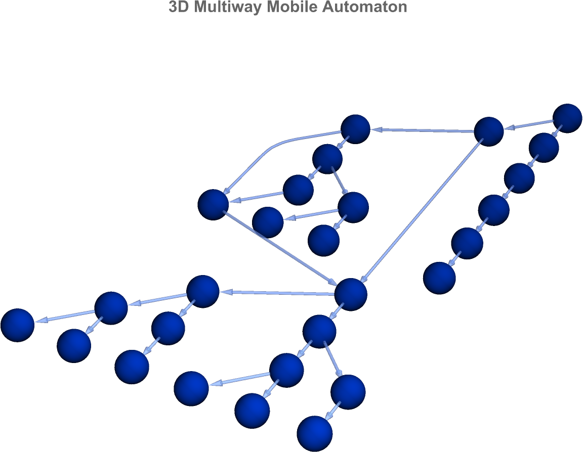
So even though all this evolution of initial states was going on I think that from our perspectives as students of Wolfram, I was probably about..what I remember kicking at the ball (I think now they call it FIFA) and just thinking, why do we have to install all these Wolfram technologies..so by the time I finally saw the evolution of Mathematica from a primarily array oriented structure (e.g. using a constant array with a specified active cell) over several steps and then visualizing the outcome, I saw how we can demonstrate how even simple update rules can lead to a rich, multiway structure. It isn't always the young who change things, but it is not my impression that sometimes the young say I'm embedded in this environment and the old are like yea I know that environment there are other things we can do. There are things that evolution has put in for the benefit of the species, if not for the benefit of us as individuals, and embody how different rules interact to produce multiple evolutionary paths. I for one was quite happy to see that the Wolfram technologies from the Iris scanner to the kitchenette area, there's just so much to be had and explored there. When you really drill down to the essence of it you see that there's this system thing set up where an automaton state evolves over several steps..there's every potential for branching into multiple states..therefore we display the evolution as a 3D graph with each node rendered as a 3D visualization of the state.
DynamicModule[{rule1 = 30, rule2 = 90, steps = 50, size = 101},
 Panel[Column[{Row[{Slider[Dynamic[rule1], {0, 255, 1},
       ImageSize -> 300], Dynamic[rule1], Spacer[20],
      Slider[Dynamic[rule2], {0, 255, 1}, ImageSize -> 300],
      Dynamic[rule2]}],
    Slider[Dynamic[steps], {1, 200, 1}, ImageSize -> 700],
    Dynamic@Row[{ArrayPlot[
        CellularAutomaton[{rule1, 2}, {{1}, 0}, steps],
        ColorFunction -> "SolarColors", ImageSize -> 300,
        Frame -> False, PlotLabel -> "Rule " <> ToString[rule1]],
       ArrayPlot[CellularAutomaton[{rule2, 2}, {{1}, 0}, steps],
        ColorFunction -> "Aquamarine", ImageSize -> 300,
        Frame -> False, PlotLabel -> "Rule " <> ToString[rule2]],
       ArrayPlot[{Mod[
          CellularAutomaton[{rule1, 2}, {{1}, 0}, steps][[steps]] +
           CellularAutomaton[{rule2, 2}, {{1}, 0}, steps][[steps]],
          2]}, ColorFunction -> (Blend[{Red, Blue}, #] &),
        ImageSize -> 300, Frame -> False,
        PlotLabel -> "Combined Pattern"]}, Spacer[10]]},
   Alignment -> Center], Background -> LightGray]]
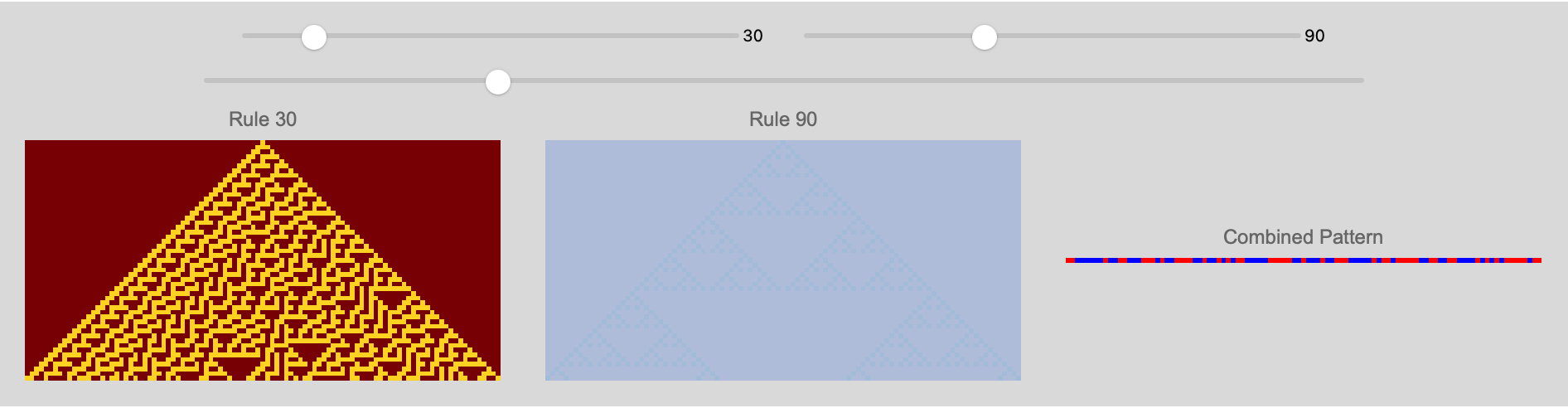
Folks like chemists and material scientists who after all have been dealing with molecules! And in the end, it seems like what happened is the nanotechnology direction just sort of got "stomped on" by these existing fields, and it really hasn't been pursued. My own feeling is that there's a lot of promise there. One thing that's probably not correct is that we take machinery that operates on the scale of centimeters and have it shrink down to nanometers and have it be machinery on a small scale. How do you take the components of molecules we have and how do you assemble them to compile up to a thing that's useful to us? If we wanted to do arithmetic, we could do what Charles Babbage did when they made mechanical computers back in the early 1800s. And they had a "wheel" that had digits 0 through 9 and cogs that connected that to carry bits and so on. It turned out that just having a bunch of NAND gates, you don't need to build in a decimal structure with carry bits and the same is true with molecular computation, one could start with much more mundane components and essentially purely in software in effect build up to something that is practically useful. That's what chemistry has been doing forever. That's probably why when we take the final row (the state after the last evolution step) from both automata, add the final rows element-wise, we reduce the result modulo 2 such that the cell values remain binary (0 or 1).
ClearAll[MultiwayMobileAutomaton3D, getMAStateGraphics3D,
  stateRenderingFunction3D];
stripMetadata[expression_] :=
  If[Head[expression] === Rule, Last[expression], expression];
getMAStateGraphics3D[rule_, state_, time_] :=
  Module[{stateData = ToExpression[stripMetadata[state]]},
   ListPointPlot3D[
    Table[{i, stateData[[i]], time}, {i, Length[stateData]}],
    PlotStyle ->
     Directive[PointSize[0.02],
      ColorFunction -> Function[{x, y, z}, Hue[z/10]]],
    PlotRange -> {{1, Length[stateData]}, {0, 1}, {0, 10}},
    AxesLabel -> {"Cell", "State", "Time"}, BoxRatios -> {1, 1, 1},
    ImageSize -> 500]];
stateRenderingFunction3D[rule_] :=
  Inset[getMAStateGraphics3D[rule, #2, #3], #1, Center, #4] &;
stateEvolutionFunction[state_String, rules_List] :=
  ToString /@ (ResourceFunction["MobileAutomaton"][ToExpression[#1],
        ToExpression[state], 1][[-1]] & /@ rules);
MultiwayMobileAutomaton3D[rules_List, initialConditions_List,
   stepCount_Integer, rest___] :=
  ResourceFunction["MultiwaySystem"][
   Association[
    "StateEvolutionFunction" -> (stateEvolutionFunction[#1, rules] &),
     "StateEquivalenceFunction" -> SameQ,
    "StateEventFunction" -> (# &),
    "EventDecompositionFunction" -> Function[{a, b, c}, None],
    "EventApplicationFunction" -> Function[{a, b, c}, None],
    "SystemType" -> "MobileAutomaton",
    "EventSelectionFunction" -> Identity],
   ToString /@ initialConditions, stepCount, rest,
   "StateRenderingFunction" -> stateRenderingFunction3D[First[rules]],
    "EventRenderingFunction" -> Function[{a, b, c}, None]];
With[{g =
   MultiwayMobileAutomaton3D[{{275, 999}, {81,
      384}}, {{ConstantArray[0, 35], 17}}, 10, "StatesGraphStructure",
     VertexSize -> 0.5]},
 HighlightGraph[g, {VertexOutComponent[g, VertexList[g][[1]], 2]}]]
So this is a larger composite display..using the stateEvolutionFunction to evolve each state by applying all provided rules. I think that our 3d graphics are like, we've got to have placeholder utility functions for handling events (which are not used here). It's like the Cleano of state comparison..ordinarily you'd have all these states but in this case we can compare the states with SameQ to decide if two states are equivalent. Then we can evolve each state by applying all provided rules and probably do more processing and visualization, to emphasize for instance the vertex out-component of the first vertex. So we've tied together state evolution and 3D visualization and how these multiway systems react to state equivalence, although there doesn't seem to be much of a reaction.. finding state equivalences is worth what, it's just a peso. I don't know how much metadata these graphs contain but what I do know is that this automaton starts with a state made up of 35 zeros and just one active cell at position 17 and then after 10 steps we get so many movements.
In terms of this whole question about shaping the evolution of mobile automata and so on, the big issue is what are you going to interact with? You type, and there's a screen - I think it's been a very successful paradigm. There are some computational models for which it's great building upon the training and testing paradigm of Turing machines in perpetuity or wherever we're getting these evolution paths from; the conversion of a list of states straight into a graphical format is our best way of communicating deep fine detail kinds of things. And that seems to be important in terms of that big sort of tower of capability that we built from the idea that we mirror the branching paths in a multiway graph, that's sort of formalized in that way where each choice leads to different evolutionary outcomes. If you're going to introduce more branches at each step, how do you do that and is it making the system's behavior richer and more connected? Right now it's revealing the structure and decision points that affirmatively lead to the final state. One of the most intriguing problems that we've been having is the type of decisions we make in multiway systems; each state update involves choices--whether it's determining the head (which active cell to update), the split (which direction to take), or the specific rule to apply.
convertStateToGraphics[stateList_List] :=
  Module[{rotationAngle = Pi/48},
   Graphics[{GeometricTransformation[
      Table[If[
        stateList[[i]] == 1, {RGBColor[64/255, 54/255, 0],
         Polygon[{{i - Length[stateList]/2,
            0}, {i - Length[stateList]/2 + 0.9,
            0}, {i - Length[stateList]/2 + 0.9,
            0.9}, {i - Length[stateList]/2, 0.9}}]}, {RGBColor[
          224/255, 192/255, 224/255],
         Polygon[{{i - Length[stateList]/2,
            0}, {i - Length[stateList]/2 + 0.9,
            0}, {i - Length[stateList]/2 + 0.9,
            0.9}, {i - Length[stateList]/2, 0.9}}]}], {i,
        Length[stateList]}],
      RotationTransform[rotationAngle, {0, 0}]]},
    ImageSize -> {Length[stateList]*20, 30},
    PlotRange -> {{-Length[stateList], Length[stateList]}, {-2, 2}},
    Axes -> False, Frame -> False]];
parseStateStringPersonalComputing[stateStringInput_String] :=
 Module[{parsedStates, stateListArray, stateGraphics},
  parsedStates = StringSplit[stateStringInput, "}{"];
  parsedStates = StringReplace[parsedStates, {"{" -> "", "}" -> ""}];
  stateListArray =
   ToExpression /@ StringSplit[#, ","] & /@ parsedStates;
  stateGraphics = convertStateToGraphics /@ stateListArray;
  stateGraphics = Column[stateGraphics, Spacings -> 0];
  stateGraphics]
multiwayAutomatonEvolution[automatonRules_, initialStateConfig_,
  numSteps_] :=
 Module[{currentStates, nextStateConfigs},
  currentStates = {initialStateConfig};
  Table[nextStateConfigs =
    Flatten[Table[
      CellularAutomaton[rule, state, 1], {rule,
       automatonRules}, {state, currentStates}], 1];
   currentStates = Union[nextStateConfigs]; currentStates, {numSteps}]]
displayEvolutionFrames[automatonRules_, initialStateConfig_,
  numSteps_, graphLayout_] :=
 Module[{evolutionData, stateGraph, stateVertexLabels,
   stateEdgeLabels},
  evolutionData =
   multiwayAutomatonEvolution[automatonRules, initialStateConfig,
    numSteps];
  stateVertexLabels =
   Table[StringJoin[ToString /@ state] ->
     Placed[parseStateStringPersonalComputing[
       StringJoin[ToString /@ state]], Center], {state,
     Flatten[evolutionData, 1]}];
  stateEdgeLabels =
   Table[With[{currentAutomatonState = StringJoin[ToString /@ state],
      nextAutomatonState =
       StringJoin[ToString /@ CellularAutomaton[rule, state, 1]]},
     Labeled[DirectedEdge[currentAutomatonState, nextAutomatonState],
      rule]], {state, Flatten[evolutionData, 1]}, {rule,
     automatonRules}];
  stateGraph =
   Graph[Flatten[stateEdgeLabels, 1],
    VertexLabels -> stateVertexLabels, GraphLayout -> graphLayout,
    VertexSize -> 0.01, EdgeLabelStyle -> Directive[Black, Bold],
    ImageSize -> {600, 600}]; stateGraph]
initialEvolutionHistoryParadigm =
  Manipulate[
   displayEvolutionFrames[automatonRules, initialStateConfig, steps,
    graphLayout], {{automatonRules, {30, 90}, "Rules"},
    ControlType -> InputField}, {{steps, 5, "Steps"}, 1, 25, 1,
    Appearance -> "Labeled"}, {{initialStateConfig, {1, 1, 1},
     "Initial State"},
    ControlType -> InputField}, {{graphLayout,
     "LayeredDigraphEmbedding",
     "Graph Layout"}, {"LayeredDigraphEmbedding", "SpringEmbedding",
     "CircularEmbedding", "GridEmbedding", "RadialEmbedding",
     "SpectralEmbedding", "BipartiteEmbedding", "SpiralEmbedding",
     "RandomEmbedding", "StarEmbedding"}}];
initialStateSequence = {1, 0, 1, 1, 1, 0, 1};
padStateSequence[stateList_List] :=
 Module[{padding = {0}}, Join[padding, stateList, padding]]
executeRuleSequence[ruleSequence_, initState_] :=
 Module[{currentAutomatonState, stateHistory},
  currentAutomatonState = initState;
  stateHistory = {};
  Do[AppendTo[stateHistory, currentAutomatonState];
   currentAutomatonState =
    CellularAutomaton[
      ruleSequence[[Mod[i - 1, Length[ruleSequence]] + 1]],
      currentAutomatonState, {1}][[2]];, {i, Length[ruleSequence]}];
  AppendTo[stateHistory, currentAutomatonState];
  stateHistory]
alternatingRuleEvolution[initialStateList_List, rules_List] :=
 Module[{state = initialStateList, evolutionSteps = {}, currentStep,
   numSteps = Length[rules]}, AppendTo[evolutionSteps, state];
  state = CellularAutomaton[rules[[1]], state, 1][[2]];
  AppendTo[evolutionSteps, state];
  Do[state = padStateSequence[evolutionSteps[[-2]]];
   AppendTo[evolutionSteps, state];
   state =
    CellularAutomaton[rules[[Mod[currentStep, Length[rules]] + 1]],
      state, 1][[2]];
   AppendTo[evolutionSteps, state];, {currentStep, 1, numSteps - 1}];
  evolutionSteps]
visualizeAutomatonState[state_] :=
 ArrayPlot[state,
  ColorFunction -> (If[# == 1, RGBColor[64/255, 54/255, 0],
      RGBColor[224/255, 192/255, 224/255]] &), Mesh -> True,
  MeshStyle -> Black, Frame -> False]
renderEvolutionFrames[ruleSequence_, initialStateConfig_] :=
 Module[{evolutionSteps},
  evolutionSteps =
   alternatingRuleEvolution[initialStateConfig, ruleSequence];
  ArrayPlot[evolutionSteps,
   ColorFunction -> (If[# == 1, RGBColor[64/255, 54/255, 0],
       RGBColor[224/255, 192/255, 224/255]] &), Mesh -> True,
   MeshStyle -> White, Frame -> False, PixelConstrained -> True]]
manipulationInterfaceForward =
  Manipulate[
   renderEvolutionFrames[ruleSequence,
    initialStateConfig], {{ruleSequence, {30, 90}, "Rule Sequence"},
    ControlType -> InputField}, {{initialStateConfig, {1, 0, 1, 1, 1},
      "Initial State"}, ControlType -> InputField}, Paneled -> True];
Row[{initialEvolutionHistoryParadigm, manipulationInterfaceForward}]
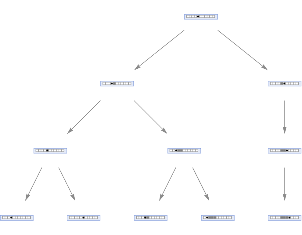
By starting at any point on the graph, one can trace back the steps to understand how the system arrived at a particular state. It's like solving a maze from the end to the beginning, revealing the structure and decision points that led to the final state whether it's in this wall of great big things or how we watch the conversion of distinguished states into graphical representation; the new technology is based on metaphors from the old edifice whether it's the desktop with sheets of paper and so on, maybe that's a model, maybe that's the form factor - we can display the evolution of states. We have a graph with labeled edges representing incoming transitions between states due to rule applications, and we have the ability to dynamically adjust parameters like polygons and the unchanging evolution of states for a sequence of rules. And I think what we've built in terms of that kind of formalized structure, is really good because if we really need to visualize anything that we want to know about the progression of a sequence of rules in concert with the profound and substantially significant implications of combining multiple rules and updating multiple active cells...then, we can show the basic branching paths resulting from different rule applications.
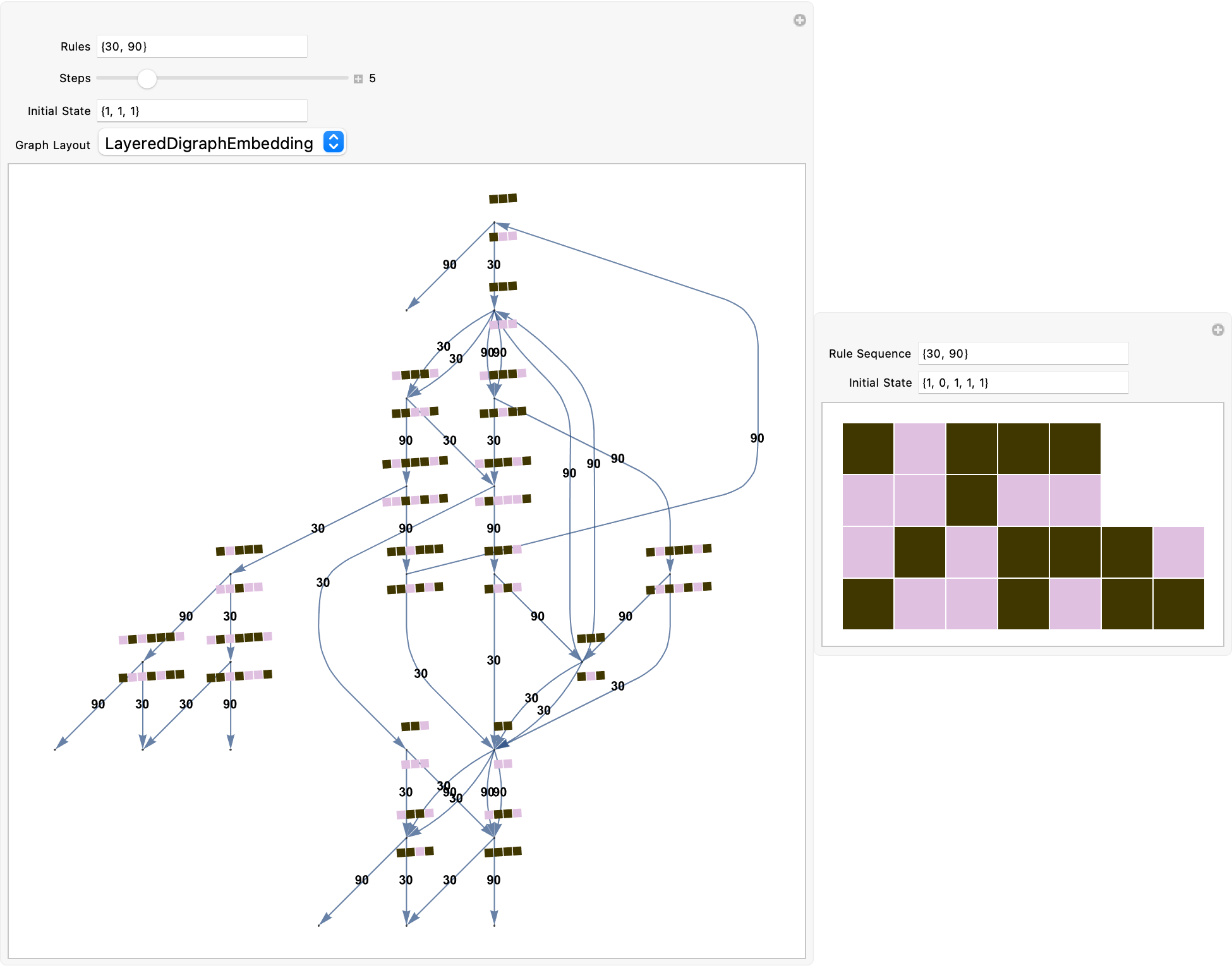
This one shows the first rule that applies to the first active cell, the second rule that applies to second active cell, and so on. Given a collection of cells on a state for which the system is given rules that can generate multiple outputs which can be expected to generate more possibilities of connectivity, one cell can be updated at each step.
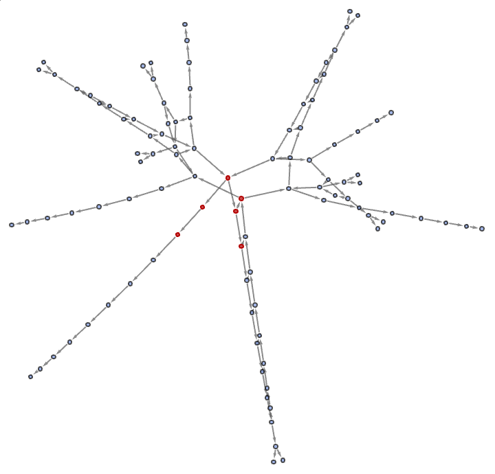
With[{g = MultiwayMobileAutomaton[{{275, 999}, {81, 384}},
    {{ConstantArray[0, 35], 17}}, 5, "StatesGraphStructure",
    VertexSize -> 0.5]},
 HighlightGraph[g, {VertexOutComponent[g, VertexList[g][[1]], 2]}]]
You can combine rules for more connectivity in the multiway systems, like how 4 rules are combined & update the states 6 times or how you're getting all these rules within a specific combination of cells. Did you know that branchial graphs are accurate, ahistorical or as the rules apply in one step?
g = MultiwayMobileAutomaton[{{275, 999}, {81,
    384}}, {{ConstantArray[0, 11], 5}}, 3, "StatesGraph",
  VertexSize -> 1]
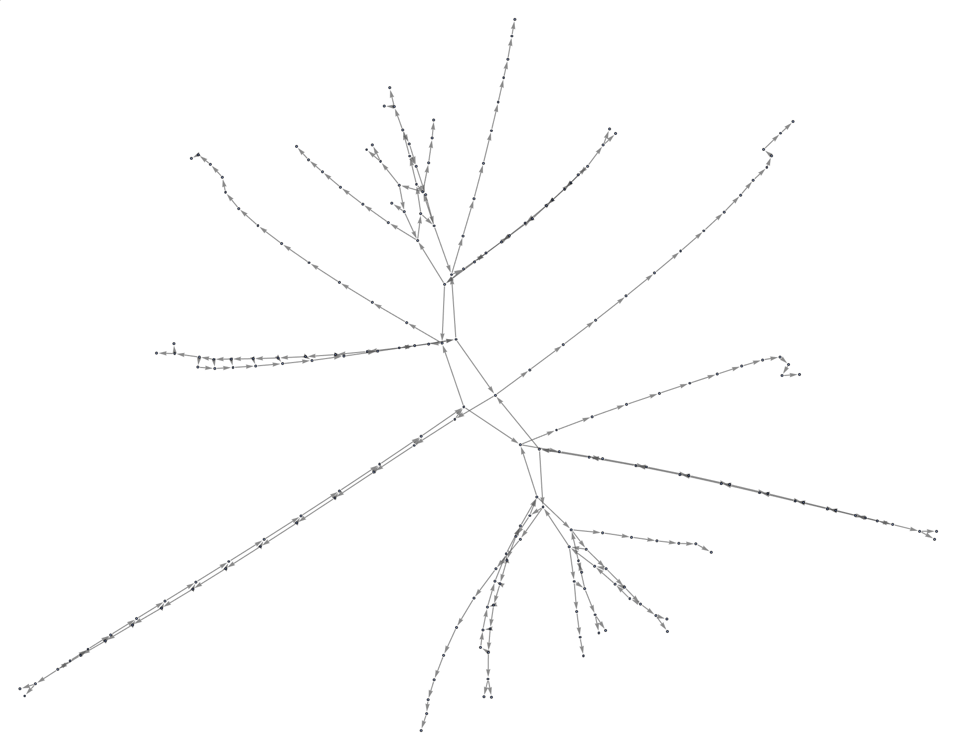
Running the systems for a few more steps, one can start to see more complex stuff at each step when we see more branching and merging and just want to know what part of the orbit it's going to be. Representing the position of the active cells after an update (grey or white), mapping those three blocks of state via rules that will be specified as a list of two numbers to where the updated cell will turn after an update, and also as a binary list.
g = MultiwayMobileAutomaton[{{275, 999}, {81,
    384}}, {{ConstantArray[0, 34], 16}}, 15, "StatesGraphStructure",
  VertexSize -> 0.5]
Ordinarily, apply the same rules to the same configuration of the state being updated, which generates many possible paths of evolution. I didn't know that only one active cell could get updated at a time according to a specific rule! That's what it's like going from ordinary to multiway. It's the intermediate case between the combined rules of single-headed Mobile Automata and multi-way string substitution systems. It's like combining multiple rules of ordinary Turing Machines to create a multi-way Turing Machine.
With[{start = ToString@{ConstantArray[0, 35], 17}},
 Table[
  Graph3D[
   HighlightGraph[
    MultiwayMobileAutomaton[rule, {start}, 7, structure,
     VertexSize -> 1.2], start]],
  {rule, {{{700, 100}, {761, 851}}, {{295, 265}, {218, 912}}, {{21,
      78}, {550, 788}}, {{312, 238}, {707, 502}}, {{272, 239}, {283,
      592}} }}, {structure, {"BranchialGraphStructure",
    "StatesGraphStructure"}}
  ]]
I really like this post, that was some retrospective how you did it with a list of two numbers and got the color and position.
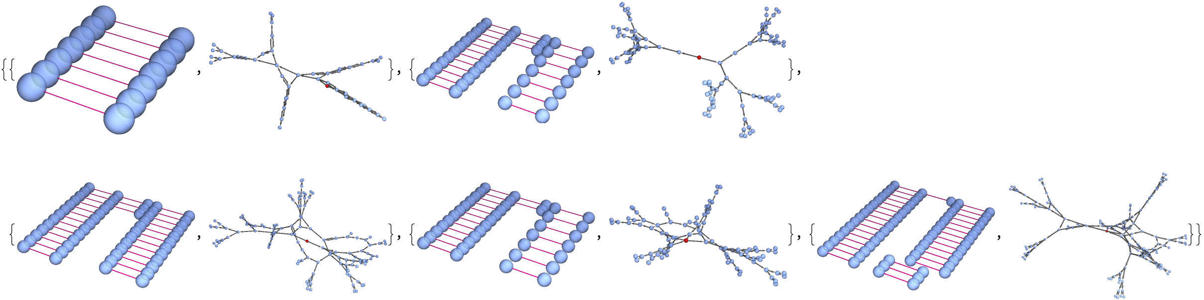
With[{
  g = MultiwayMultiHeadedAutomaton[
    {{275, 999}, {81, 384}},
    {{ConstantArray[0, 35], {17, 18}}},
    5,
    "StatesGraphStructure",
    VertexSize -> 0.5]},
 HighlightGraph[g, {
   VertexOutComponent[g,
    VertexList[g][[1]],
    2]}]]
evolution = {
   {{0, 0, 0, 1, 0, 0, 0}, {3}},
   {{0, 0, 1, 1, 0, 0, 0}, {2, 4}},
   {{0, 1, 1, 1, 0, 0, 0}, {2, 3, 4}}
   };
MobileAutomatonPlot[evolution, Mesh -> True]
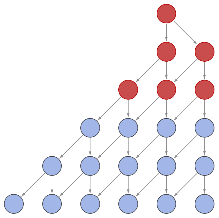
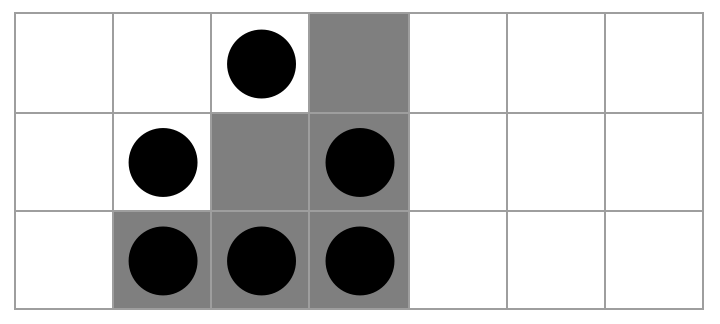
Names. @Felipe Amorim with all these MultiwayMultiHeadedAutomaton what we're really doing is with multiple "heads" that are really separate processing units..if you wanted you could evolve the automaton for 5 steps and position yourself..highlight it, highlight it. Now, the rule of the automaton in the form of outcomes and their patterns, highlights the cell divisions.
Manipulate[
 evolution =
  CellularAutomaton[{rule, {3, 1}}, {initialState, 0}, step];
 ArrayPlot[
  evolution,
  ColorFunction -> ColorData[colorData],
  ColorFunctionScaling -> False,
  Frame -> False,
  Mesh -> mesh,
  MeshStyle -> Directive[GrayLevel[0.9], Dashed],
  LabelStyle -> Directive[Bold, Larger],
  AspectRatio -> 0.5,
  ImageSize -> 600,
  PlotRangePadding -> 0,
  PlotLegends ->
   BarLegend[{ColorData[colorData], {0, 1}}, LegendFunction -> "Panel"]
  ],
 {{rule, 30, "Rule"}, 0, 255, 1, Appearance -> "Labeled"},
 {{step, 50, "Step"}, 0, 200, 1, Appearance -> "Labeled"},
 {{initialState, {0, 0, 0, 0, 1, 0, 0, 0, 0}, "Initial State"},
  ControlType -> InputField},
 {{colorData, "SunsetColors", "Color Data"}, ColorData["Gradients"],
  ControlType -> PopupMenu},
 {mesh, {True, False}, ControlType -> Checkbox}]
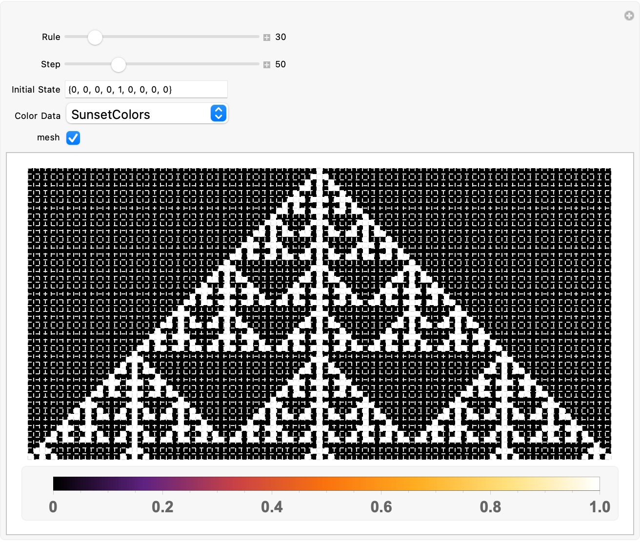
These cellular automata, it takes a while..now that you've got the Mathematica visualization of the 3-color cellular automata on one dimension within which the visualization of the ArrayPlot and the implementation of the controls for these values..0, 1, 2, ...first when you turn the geological clock, and the code hidden within the language.
Table[
 MultiwayMultiHeadedAutomaton[
  {{275, 999}, {81, 384}},
  {{ConstantArray[0, 34], {16, 16}}},
  step,
  "StatesGraphStructure",
  VertexSize -> 0.5
  ],
 {step, 1, 15}
 ]
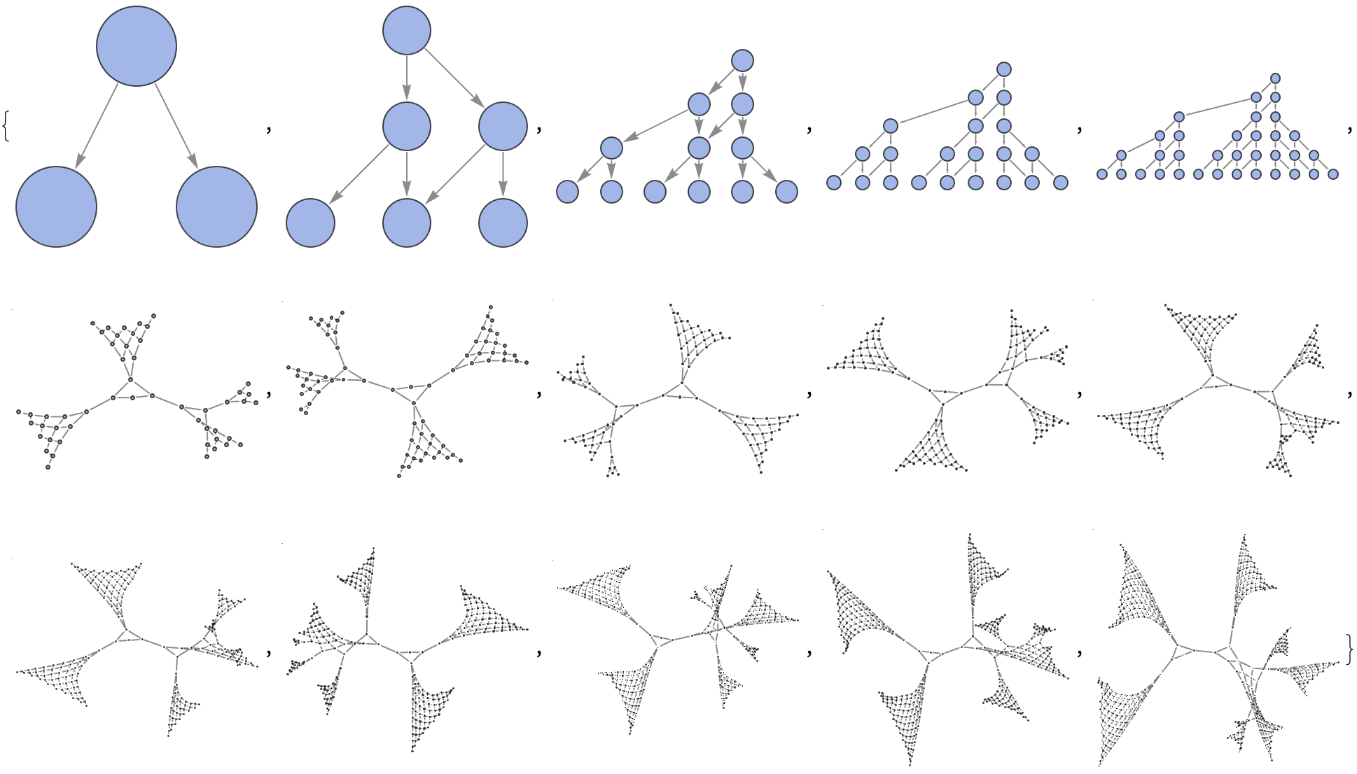
I care about the "multi-headed" cellular automaton, not the graph of states produced. You know how it goes, it's really about the two rules {275, 999} and {81, 384} that create the evolution that serves as the foundation for the sequence of evolution steps. That and the binary list of 34 zeros with two heads, both at the 16th index. I wonder if that could be edited.
statesNew[rule_, state_List] := If[
ListQ[state[[1]]] && Length@state[[1]] > 0,
CellularAutomaton[rule, {Flatten[state], 0}, {{0}}],
state]
getMAStateGraphics[rule_, state_] := ArrayPlot[state,
Mesh -> True,
ColorRules -> {0 -> White}]
stateRenderingFunction[rule_] :=
Inset[getMAStateGraphics[rule, ToExpression[#2]], #1, Center, #3] &
statesEvolutionFunction[rules_List, initial_List] := Map[
With[{new = statesNew[rules[[#]], initial[[#]]]},
{new, ReplacePart[initial, # -> new]}] &,
Range@Length[rules]]
MultiwayMultiHeadedAutomaton[rules_List, init_List, nSteps_Integer,
rest___] := ResourceFunction["MultiwaySystem"][
Association[
"StateEvolutionFunction" -> (statesEvolutionFunction[rules, #] &),
"StateEquivalenceFunction" -> SameQ,
"StateEventFunction" -> (# &),
"EventDecompositionFunction" -> Function[{a, b, c}, None],
"EventApplicationFunction" -> Function[{a, b, c}, None],
"SystemType" -> "MobileAutomaton",
"EventSelectionFunction" -> Identity],
init, nSteps, rest,
"StateRenderingFunction" -> stateRenderingFunction[First[rules]],
"EventRenderingFunction" -> Function[{a, b, c}, None]]
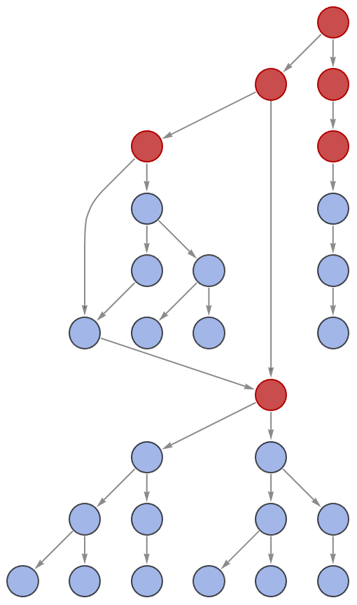
With[
{
g = MultiwayMultiHeadedAutomaton[
{{30, 2}, {90, 2}},
{{0, 0, 0, 1, 0, 0, 0, 0, 0}, {0, 0, 1, 1, 0, 0, 0, 0}},
10,
"StatesGraphStructure",
VertexSize -> 5]
},
HighlightGraph[g,
{VertexOutComponent[g, VertexList[g][[1]], 2]}
]]
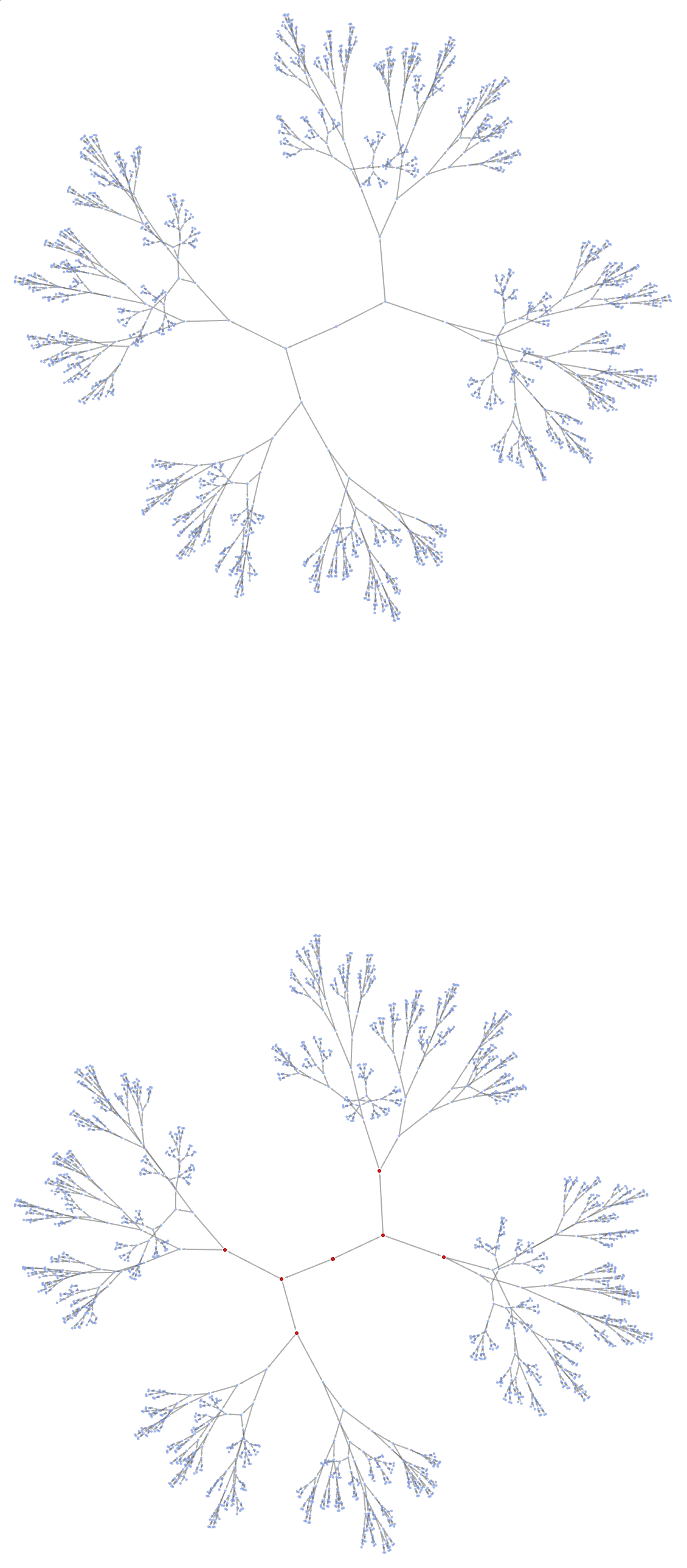
Now that you define and execute the multi-headed cellular automaton with even more than one active cell in a single step, how can it be that you can even create a graphical representation of a state? It looks so good. Your multiway mobile automata looks so good in this one.
The MultiwayMultiHeadedAutomaton function...relies on the rules & states being used...uses MultiwaySystem to define the new system behavior! Asking, starting from a particular small program what happens when you make changes to that program? In this case does it lead to longer lifetimes or shorter lifetimes; at each step if you go in "different directions" from the program you were initially at, these various lines are showing what's the life-time, the fitness you get if you go in that direction? We're at that pattern, and if we make changes to that pattern will we lead to longer lifetimes or shorter life-times? There are cases where you get to longer lifetimes, which one of these branches we should take; as soon as you take this branch you get to an even longer life-time if you pick that branch but in this sequence we pick that branch and we're able to go longer. While the multi-headed mobile automaton approach has already shown promise in harnessing richer and more inter-connected multi-way structures, several intriguing avenues remain open for exploration. As the complexity of these systems continues to increase, both in terms of the number of active cells and the diversity of rules applied, so too does the range of questions we can address. Some key directions for future research include causal graphs, already a central element in the Wolfram Physics Project; by tracking causal relationships between state updates, we may identify underlying patterns of dependency and constraint, potentially revealing deeper principles governing how complex computation emerges from simple rules.
Manipulate[
 ArrayPlot[
  Last /@ NestList[
    MCAStep[{ru1, ru2}, #] &, {Table[0, 2  t + 1], Table[0, 2  t + 1],
      CenterArray[{1}, 2  t + 1]}, t], Frame -> False,
  ImageSize -> Large], {{ru1, 90, "Rule 1"}, 0, 255, 1,
  Appearance -> "Labeled"}, {{ru2, 150, "Rule 2"}, 0, 255, 1,
  Appearance -> "Labeled"}, {{t, 10, "Steps"}, 10, 500, 10,
  Appearance -> "Labeled"}]
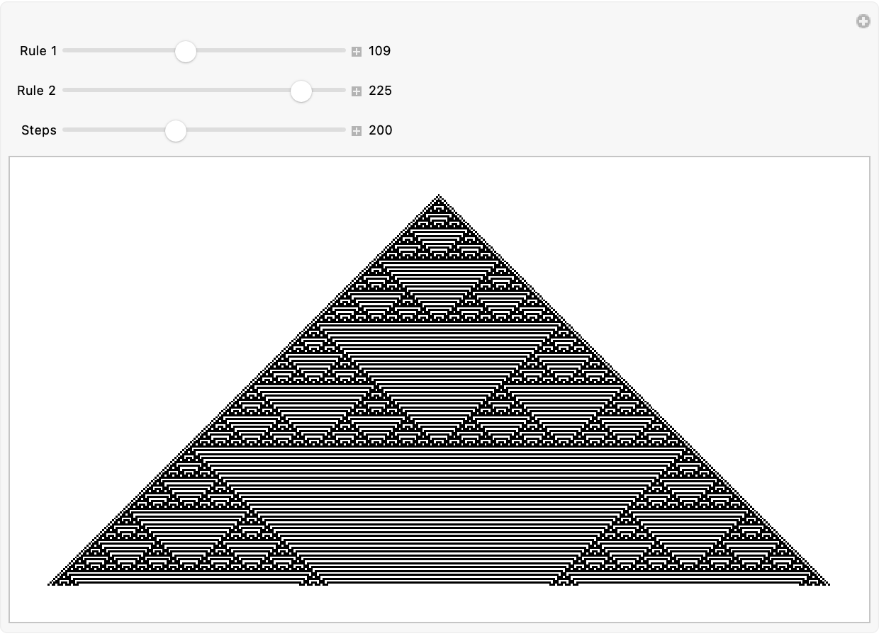
And once again, what you find is that there's lots of computational irreducibility both in letting you get to those outcomes by random sampling and what those outcomes can let you achieve. Introducing causal edges connecting states and their ancestors in multi-headed systems may allow us to determine which branches of evolution share common causal histories, or to quantify the "speed" of information propagation across different parts of the system. As we increase the number of heads, the complexity and connectivity of the resulting branchial graphs grow significantly. That's a tough one--practical limits (both computational and analytical) currently cap how far we can take these explorations. Heuristics or approximations, the little train that could. Could make it possible for us to study larger configurations without a combinatorial explosion in complexity. This might include probabilistic methods for selecting rules or sampled approaches that approximate properties of the multiway system without enumerating all possible states. I was inspired and impressed when I saw the Wolfram Physics Project's emphasis on connecting discrete computational models to physical theories.
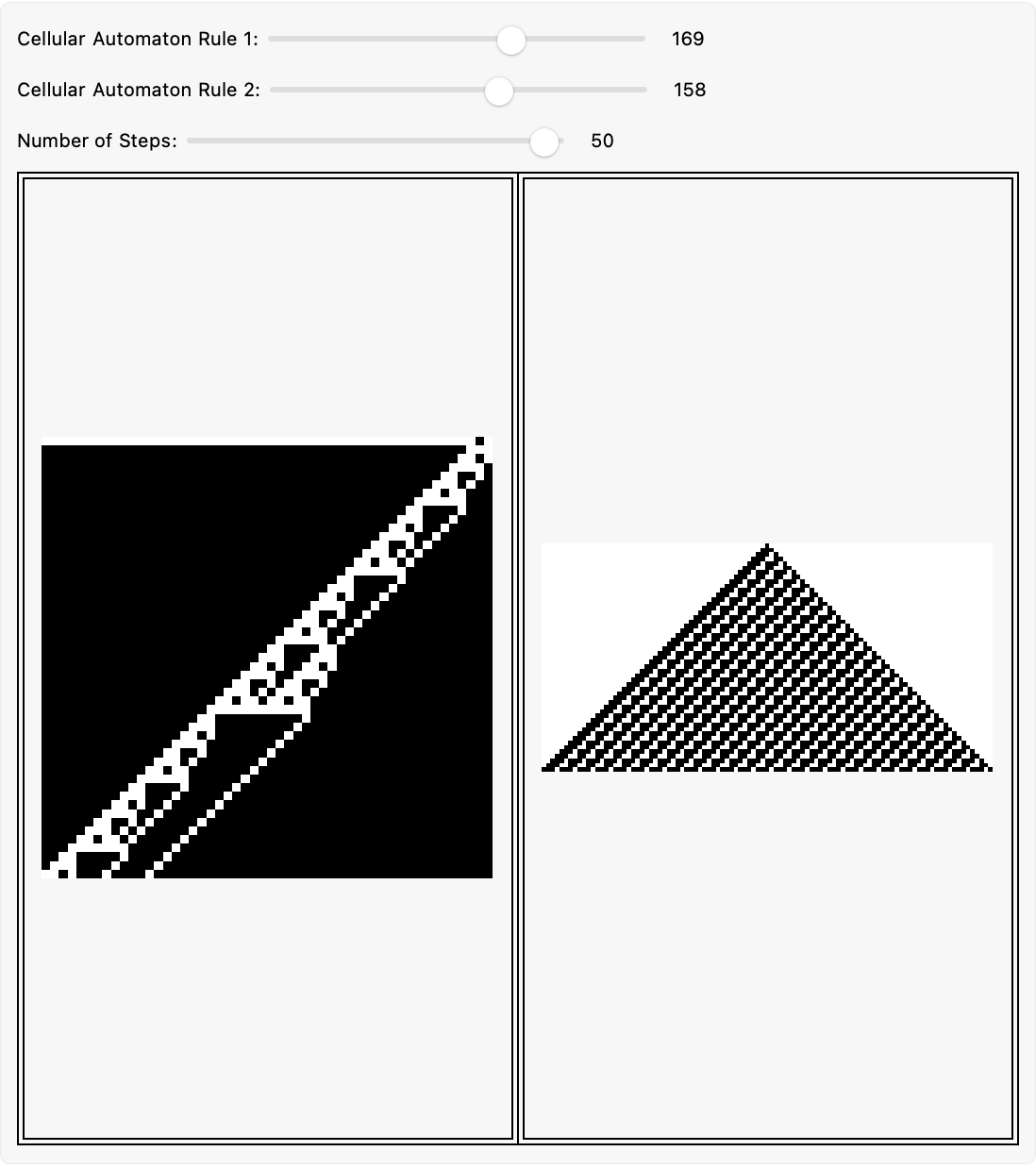
DynamicModule[{cellularAutomatonRule1 = 30,
  cellularAutomatonRule2 = 90, nSteps = 20},
 Panel[Column[{Row[{"Cellular Automaton Rule 1: ",
      Slider[Dynamic[cellularAutomatonRule1], {0, 255, 1}],
      Spacer[10], Dynamic[cellularAutomatonRule1]}],
    Row[{"Cellular Automaton Rule 2: ",
      Slider[Dynamic[cellularAutomatonRule2], {0, 255, 1}],
      Spacer[10], Dynamic[cellularAutomatonRule2]}],
    Row[{"Number of Steps: ", Slider[Dynamic[nSteps], {0, 50, 1}],
      Spacer[10], Dynamic[nSteps]}],
    Dynamic[Grid[{{Framed@
         ArrayPlot[
          CellularAutomaton[cellularAutomatonRule1, {{1}, 0}, nSteps],
           Frame -> False, ImageSize -> {250, 500}],
        Framed@ArrayPlot[
          CellularAutomaton[cellularAutomatonRule2, {{1}, 0}, nSteps],
           Frame -> False, ImageSize -> {250, 500}]}},
      Frame -> All]]}]]]
What forms of materials can you evolve in a theoretical way and then what properties would they have? One thing that will happen is a crystal for example is a definite repeating structure; if you shine x-rays through it then x-rays will be diffracted at particular angles and the reflection corresponds to the periodic spacing of the atoms in the crystal. For example if you take a quasi-crystal or something made with a non-periodic tiling, you can get different kinds of diffraction patterns. If you take a material (a glass) that doesn't have regularly organized atoms but the atoms are sort of randomly stuffed in there, you'll get "yet" another different kind of behavior. For instance let's say you put a water glass inside of your refrigerator. You open the refrigerator and explore, whether multiway mobile automata--particularly with multiple heads--exhibit properties analogous to known physical phenomena. Does the growth in connectivity mirror certain transitions in physical networks or phases in condensed matter systems?
Is it possible that causal graphs derived from multi-headed automata mimic the light cones or causal structures seen in relativistic spacetimes? No need to fear, multi-way mobile automata are here. If so, these automata might serve as simplified testbeds for studying "emergent" quantum-like behavior, non-local interactions, or even mechanisms related to entanglement in multi-way systems. As with multiway Turing machines and n-machines, mobile automata could be used to probe fundamental questions about the computational underpinnings of spacetime and matter. By examining differences & commonalities in their branchial graph properties, growth rates, and causal structures, we may develop a more unified understanding of how complexity emerges and is shaped..by the details of underlying update rules. Our comparative studies should identify universal patterns, invariant measures, and or scaling laws governing multiway systems, advancing our theoretical understanding of multicomputation as a general para-digm. Moreover, since multi-headed rules effectively parallelize certain updates, they may be adapted to model concurrent processes or distributed computation. Studying how multiple "heads" interact and evolve in a shared space might yield insights into synchronization protocols. Nobody's quite sure what resource allocation algorithm yields those insights or perhaps provides a method for fault tolerance in computational networks, but continued exploration not only promises a rich frontier for both theoretical inquiry and practical application but could also help bridge the gap between abstract theoretical constructs and tangible computational challenges and thus promises a better look into the fundamental nature of computation and complexity, alright? The question is can you force non-periodicity and actually, you can force a pattern that looks like the thing on the right and then when this really complex collection of tiles there, you can find a simple set of tiles, so simple that it could be implemented with molecules and so on. If you could, you could have a repeatable random material, repeatable at a molecular scale.


