The Mathematical Storytelling that's like what I need Linguistic Leaps and Bounds because this is some effective pedagogy that eases the transition for students from high-school to college-level, the QA forms that give us the language of the discipline of mathematical epidemiologists as they examine the effects of these parameters, of infectious disease spread. @Lybrya Kebreab.

ClearAll[s, e, i, t, \[Lambda], \[Beta], \[Mu], \[Alpha], \[Gamma], \
\[Delta]]
sliderRow[label_, dynamicVar_, {min_, max_}] := Row[{
    label,
    Spacer[5],
    Dynamic[dynamicVar],
    Spacer[20],
    Slider[
     Dynamic[dynamicVar],
     {min, max},
     Appearance -> "Labeled"
     ]}];
DynamicModule[{s0 = 0.6, e0 = 0.7, i0 = 0.5, ttime = 5},
 Column[{
   sliderRow["\[Lambda] =", \[Lambda], {0, 2}],
   sliderRow["\[Beta] =", \[Beta], {0, 1}],
   sliderRow["\[Mu] =", \[Mu], {0, 1}],
   sliderRow["\[Alpha] =", \[Alpha], {0, 1}],
   sliderRow["\[Gamma] =", \[Gamma], {0, 1}],
   sliderRow["\[Delta] =", \[Delta], {0, 1}],
   Row[{Dynamic[
      sol = NDSolve[{

         s'[t] == \[Lambda] - \[Beta] s[t] - \[Mu] s[t] + \[Alpha] i[
             t], e'[t] == \[Beta] s[t] - (\[Gamma] + \[Mu]) e[t], 
         i'[t] == \[Gamma] e[t] - (\[Alpha] + \[Mu] + \[Delta]) i[t],
         s[0] == s0, e[0] == e0, i[0] == i0}, {s, e, i}, {t, -ttime, 
         ttime}];
      Plot[Evaluate[
        {s[t], e[t], i[t]} /. sol],
       {t, -ttime, ttime},
       PlotLegends -> {"s[t]", "e[t]", "i[t]"},
       PlotStyle -> ColorData["DarkRainbow"] /@ Range[0, 1, 1/3],
       ImageSize -> 400,
       BaseStyle -> {FontColor -> Yellow}
       ]
      ],
     Dynamic[
      ParametricPlot3D[
       Evaluate[{s[t], e[t], i[t]} /. sol],
       {t, -ttime, ttime},
       BoxRatios -> {1, 1, 1},
       AxesLabel -> {"s", "e", "i"},
       PlotRange -> All,
       ImageSize -> 400,
       BaseStyle -> {FontColor -> Yellow}
       ]]},
    Background -> RGBColor[0.2, 0.1, 0.2]
    ]
   }]]

The Wolfram Language vector fields and linear transformations absolutely show what we're looking for. I developed a positive mathematics identity. It begs the question of the good meta-model for the observer, abstracting away the computer system. @Lybrya Kebreab that was the best instructional experience that I have ever had. That was more than I could have ever deserved. It was like showing a three year old everything there is to know about the elements of a Turing Machine. Because I learned so much just from making connections within & among dynamic representations of the differential equations and the dynamics of infectious disease spread.

But now these prompts give us this structural transport between these different areas of Mathematics, the authentic historical context that allows us to engage in and build methods to understand how a Supernova spreads out.

Happy Holidays! It's been a while so I decided to check Wolfram land. And what we've got is this intersection of language and computational tools, it's fantastic, you can build up our mathematical understanding whether it's from high school to college-level mathematics. The goal of course is to emphasize and encourage the usage of Wolfram Language because that's the best thing that we can do. The real question of course is what are things like from the teaching process side of the angle, when we're building up the strength of this conceptual foundation that allows us to raise adoption of the Wolfram Language what with all these pedagogical, detailed incorporations of your methodology into the Wolfram Community.

Manipulate[
 Module[
  {solution, susceptible, infected, exposed, recovered},
  solution = NDSolve[{
     susceptible'[t] == -beta*susceptible[t]*infected[t] + lambda - 
       mu*susceptible[t],
     exposed'[t] == 
      beta*susceptible[t]*infected[t] - (sigma + mu)*exposed[t],
     infected'[t] == 
      sigma*exposed[t] - (gamma + mu + delta)*infected[t],
     recovered'[t] == gamma*infected[t] - mu*recovered[t],
     susceptible[0] == s0,
     exposed[0] == e0,
     infected[0] == i0,
     recovered[0] == r0},
    {susceptible, exposed, infected, recovered},
    {t, 0, maxTime},
    Method -> "StiffnessSwitching"];
  Plot[
   Evaluate[{susceptible[t], exposed[t], infected[t], recovered[t]} /. 
     First[solution]],
   {t, 0, maxTime},
   PlotStyle -> {
     Directive[RGBColor[0, 0, 0], Thickness[0.005]],
     Directive[RGBColor[1, 0, 1], Dashed, Thickness[0.005]],
     Directive[RGBColor[1, 1, 0], DotDashed, Thickness[0.005]],
     Directive[RGBColor[0, 1, 1], Dotted, Thickness[0.005]]},
   PlotLegends -> Placed[
     LineLegend[
      {"Susceptible", "Exposed", "Infected", "Recovered"},
      LegendMarkers -> None,
      LegendLayout -> "Column",
      LabelStyle -> {FontSize -> 14}],
     Right],
   AxesLabel -> {"Time", "Population"},
   AxesStyle -> Directive[FontSize -> 14, FontFamily -> "Arial"],
   PlotRange -> All,
   PlotTheme -> "Scientific",
   ImageSize -> Large,
   Frame -> True,
   FrameStyle -> Directive[Black, 12],
   GridLines -> Automatic,
   GridLinesStyle -> Directive[Gray, Dashed]]],
 {{beta, 0.3, "Transmission Rate (\[Beta])"}, 0, 1, 
  Appearance -> "Labeled"},
 {{sigma, 0.1, "Exposure Rate (\[Sigma])"}, 0, 1, 
  Appearance -> "Labeled"},
 {{gamma, 0.05, "Recovery Rate (\[Gamma])"}, 0, 1, 
  Appearance -> "Labeled"},
 {{delta, 0.01, "Disease-Induced Death Rate (\[Delta])"}, 0, 1, 
  Appearance -> "Labeled"},
 {{mu, 0.01, "Natural Death Rate (\[Mu])"}, 0, 1, 
  Appearance -> "Labeled"},
 {{lambda, 0.01, "Population Growth Rate (\[Lambda])"}, 0, 1, 
  Appearance -> "Labeled"},
 {{s0, 0.99, "Initial Susceptible"}, 0, 1, Appearance -> "Labeled"},
 {{e0, 0.0, "Initial Exposed"}, 0, 1, Appearance -> "Labeled"},
 {{i0, 0.01, "Initial Infected"}, 0, 1, Appearance -> "Labeled"},
 {{r0, 0.0, "Initial Recovered"}, 0, 1, Appearance -> "Labeled"},
 {{maxTime, 100, "Time Span"}, 1, 200, Appearance -> "Labeled"},
 TrackedSymbols :> {beta, sigma, gamma, delta, mu, lambda, s0, e0, i0,
    r0, maxTime}
 ]

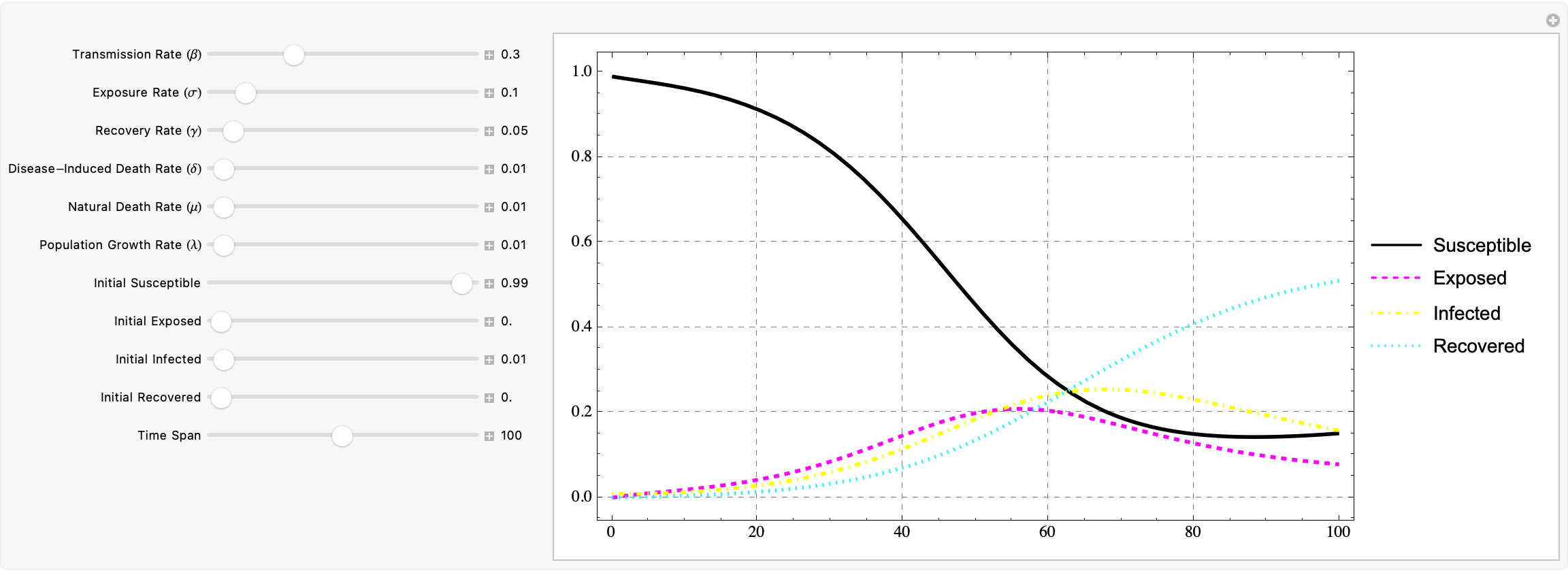
What this does is, it quickly creates an interactive simulation which allows us to dynamically model the dynamics..of an epidemic, using a compartmental model in epidemiology. The significance of compartmentalizing the population into four divisions could not be made more clear; let's say we're susceptible to some infections like the seasonal flu, which would have a basic reproduction number of 1.2 for which the infectious period would be about 5 days which translates to 0.2 per day...therefore 1.2 * 0.2 would be 0.24 per day. Just because we have these values doesn't mean we can't use them; now I don't know how these diseases get transmitted but let's say we've got some data on measles, which is highly contagious by the way, we're going to take the lower bound of the basic reproduction number so we get 12 * 0.14 (since day to day the infectious period is approximately 7 days, so 1/7 days is 0.14 per day)... or let's say we take Smallpox. Okay, so smallpox you get something like 5 * 0.083 = 0.415, to say the least. Now, how long does it take to recover from these diseases? I think the most important thing and this is so important, the fact that we have these diseases might imply something outside of the way that these disease recoveries are traditionally explained; using an average duration of 6 days we're going to get 0.17 per day for the flu, 1/8.5 days for measles, and 1/13 days for smallpox. That's to say nothing about the mortality or severity of the disease.

And so for the initial proportions of the population we've got in each of the four compartments, we can create an interactive display of the scenario in which we have four choices, it's similar to web design in that these parameters, the transmission rate can be a direct measure of how often susceptible individuals come into contact with infected ones, that's beta, and then we have the exposure rate - this is the rate at which the exposed individuals become infected, that's sigma - and then we have the gamma, the recovery rate, which tells us the rate at which infected individuals recover or die, and this is the important thing; the disease-induced death rate delta, which can be considered as just another part of the transition from infected to recovered...I think some of these can be deleted though, we've got the natural death rate mu, which affects all compartments..the idea is that we have this continuous population growth against all of these components..it's sort of like building the head section of a website that contains metadata, mastheads and calls to action, I think I experienced something similar with parameterization when using SheetMonkey to interface with Google Maps. Google Analytics is the best what with all those backend Python scripts, anyway.

And this is why it's so important to design some of these modals so that we can teach stuff such as, how do you find the Taylor series of a function for hundreds of polynomials..it's really a matter of incorporating computational communication onto our understanding of bijective, complex systems, such as the spread of infectious diseases, through differential equations and dynamic modeling. That's how Ramanujan did it what with the narrative of the Trinidad and Tobago typhoid fever outbreak narrative that you've got there. But that's all water under the bridge. If we can see the relevance of the mathematical theory in practical applications, then we can allow students to contextualize their learning.

numberSystemStyleSheet := {
   PlotRange -> {{-10, 10}, All},
   AxesLabel -> {"x", "f(x)"},
   ImageSize -> 400,
   PlotTheme -> "Scientific",
   PlotStyle -> Thick,
   LabelStyle -> {FontFamily -> "Helvetica", 12},
   Frame -> True,
   ImagePadding -> {{Automatic, Automatic}, {Automatic, 30}},
   FrameStyle -> Directive[FontSize -> 12],
   GridLines -> Automatic,
   GridLinesStyle -> Directive[GrayLevel[0.7], Dashed],
   Background -> Directive[Opacity[0.1], GrayLevel[0.95]]
   };
plotLabel := 
  Style["Interactive Storytelling Module for Understanding Limits and \
Derivatives", Bold, 14];
subtitle := 
  "Welcome to the Journey of Calculus! Follow the story to learn \
about limits and derivatives.";
successorForm1[] := Labeled[
   Column[{
     TextCell[
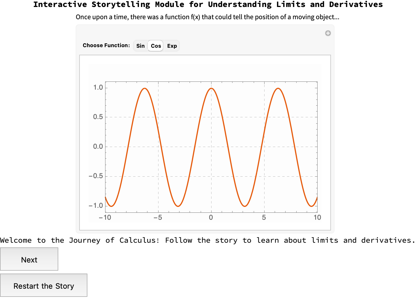
      "Once upon a time, there was a function f(x) that could tell \
the position of a moving object...", "Text", FontSize -> 12],
     Manipulate[
      Plot[function[t], {t, -10, 10}, 
       Evaluate[numberSystemStyleSheet]],
      {{function, Sin, "Choose Function:"}, {Sin -> "Sin", 
        Cos -> "Cos", Exp -> "Exp"}},
      LabelStyle -> Bold,
      ControlPlacement -> Top]}],
   {plotLabel, subtitle},
   {Top, Bottom}
   ];
successorForm3[] := Labeled[
   Column[{
     TextCell[
      "They discovered that by examining the rate of change, they \
could predict the function's behavior at any point!", "Text", 
      FontSize -> 12],
     Manipulate[
      Show[
       Plot[fn[t], {t, -10, 10}, Evaluate[numberSystemStyleSheet]],
       Graphics[
        {Thickness[0.01], Purple, 
         Line[{{x, fn[x]}, {x + slopeHeight, fn[x + slopeHeight]}}]}]],
      {{x, 0, "x:"}, -10, 10},
      {{slopeHeight, 0.1, "Slope Height:"}, 0.01, 1},
      {{fn, Sin}, None}, LabelStyle -> Bold, 
      ControlPlacement -> Top]}],
   {plotLabel, subtitle},
   {Top, Bottom}
   ];
successorForm2[] := Labeled[
   Column[{
     TextCell[
      "To predict the future, the wise mathematicians of the land \
would observe the function as x approached a certain value...", 
      "Text", FontSize -> 12],
     Manipulate[
      Show[
       Plot[fn[t], {t, -10, 10}, Evaluate[numberSystemStyleSheet]],
       Graphics[{Purple, PointSize[Large], Point[{x, fn[x]}]}]],
      {{x, 0, "Approach Value x:"}, -10, 10, 
       Appearance -> "Labeled"},
      {{fn, Sin}, None}, LabelStyle -> Bold, 
      ControlPlacement -> Top]}],
   {plotLabel, subtitle},
   {Top, Bottom}
   ];
successorForm4[] := Labeled[
   Column[{
     TextCell[
      "And thus, they mastered the magic of derivatives, which \
allowed them to foresee the path of any function!", "Text", 
      FontSize -> 12],
     Manipulate[
      Plot[{fn[t], derivativeFn[t]}, {t, -10, 10}, 
       Evaluate[numberSystemStyleSheet], AspectRatio -> 1/GoldenRatio],
      {{fn, Sin, "Function:"}, {Sin -> "Sin", Cos -> "Cos", 
        Exp -> "Exp"}},
      {{derivativeFn, Cos, 
        "Derivative:"}, {Cos -> "Cos", -Sin -> "-Sin", 
        Exp -> "Exp"}},
      LabelStyle -> Bold,
      ControlPlacement -> Top]}],
   {plotLabel, subtitle},
   {Top, Bottom}
   ];
DynamicModule[{storyForm = 1},
 Column[{
   Dynamic[
    Which[
     storyForm == 1, successorForm1[],
     storyForm == 2, successorForm2[],
     storyForm == 3, successorForm3[],
     storyForm == 4, successorForm4[]],
    TrackedSymbols :> {storyForm}],
   Button[
    "Next",
    If[storyForm < 4, storyForm++, storyForm = 1],
    ImageSize -> {100, 40},
    Appearance -> "FramedPalette"],
   Button[
    "Restart the Story",
    storyForm = 1,
    ImageSize -> {150, 40},
    Appearance -> "FramedPalette"]}],
 Initialization :> (fn = Sin; successorFn = Cos;)]

I think in order to convey the idea of the concept of the rate of change, we start out with an interactive plot. Not because it is easy, but because it actually allows us to choose between different functions (Sin, Cos, Exp) to see their graphs. Then, we can progress to the next concept which is the concept, of limits. If we can move a point along the graph of the chosen function to understand how the function behaves as x approaches certain values, then we can fully explore the concept of limits..and then we can do the rate of change via the visual aid of the visualization of slope. Last but not least there's the graph of the function that we get with its derivative, so that we can graphically portray things. This interactive, narrative-driven approach spins the educational narrative around 180 degrees, actually highlighting the importance of slowing down the instructional pace. It's not just designing SAT flashcards or demonstrating comprehension of high school to college-level mathematics. No matter what we choose as students, we want to advocate for a student-centered learning environment and I know there are all these layers of health and disease conditions that don't necessarily match up, why reinvent the wheel? We can directly translate our mathematical knowledge into computational knowledge. Remember there are mathematical equations that relate some function with its derivatives, and in this case we can model the change in disease status, within a population, over time.

And that's why we have these pedagogical strategies, they always say slow down. And I think that's a helpful technique. But it doesn't pay to just incorporate historical contexts and computational tools to create this kind of immersive experience, you've also got to articulate them and manipulate the mathematical concepts so that we can prepare students for advanced studies and applications in mathematics, and the power tower of derivative fields as they get titrated, the pedagogical approach is about a way of thinking in an organized fashion about the world.

DynamicModule[
 {aValues, b, c, quadraticPlots, y0, sol, differentialPlots},
 aValues = Range[-2, 2, 0.5];
 b = 1;
 c = 1;
 quadraticPlots = Table[
   Plot[
    a x^2 + b x + c,
    {x, -10, 10},
    PlotRange -> {-10, 10},
    PlotStyle -> ColorData["SouthwestColors"][(a + 2)/4]],
   {a, aValues}
   ];
 y0 = 0;
 differentialPlots = Table[
   sol = 
    DSolveValue[{y'[x] == a y[x]^2 + b y[x] + c, y[0] == y0}, y, x];
   {
    ColorData["Rainbow"][(y0 + 10)/20],
    Plot[sol[x],
     {x, -10, 10},
     PlotRange -> {-10, 10},
     AxesLabel -> {"x", "y"},
     PlotStyle -> ColorData["SouthwestColors"][(y0 + 10)/20]]},
   {y0, -10, 10, 2}];
 Column[
  {
   TextCell["Explore ax^2 + bx + c for various signature values of a"],
   Show[quadraticPlots, PlotRange -> All, ImageSize -> Large],
   Button["Discuss",
    CreateDialog[{
      TextCell[
       "Reflect on the impact of each parameter on the graph's \
shape."],
      DefaultButton[]}]]}],
 Initialization :> {b = 1, c = 1}]

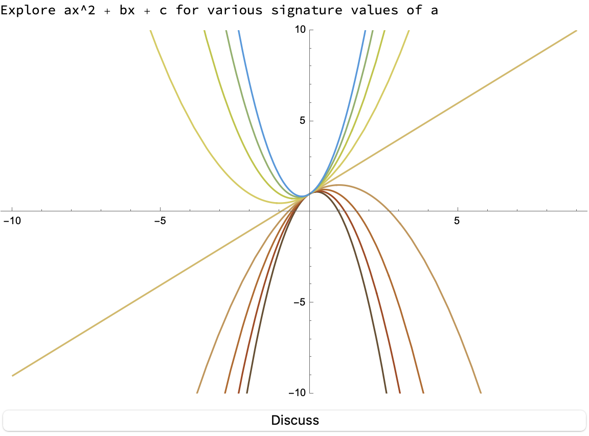
And, anybody who's been a educator for long enough would know what it means to teach such a sophisticated computational language, the Wolfram Language variety that is used in Mathematica; teaching doesn't have to preclude all manners of things like instructing a cat on how to jump, or how to meow louder and emulate the sound of human voices..I think all of this computational hype has a lot to do with where we are at the intersection of mathematics education, computational technology, and effective communication. Especially in epidemiology, where complex mathematical concepts exist out of which can be made plots of polynomial functions that can provide visual insights into their behavior. What if we want to create an interactive module exploring the number and nature of roots and the end behavior? How does understanding polynomials involve finding their roots? Even if we find the solutions to the equation formed, set the polynomial equal to zero, we haven't got the technique yet of say, breaking down polynomials into irreducible factors..we've got to understand these fundamental properties and I think that's why it's so important to make the transition to computational methods via the use of the Wolfram language for mathematical discourse. If we have the polynomial equations we can explore them using the computational software of the future that allows us to manipulate and visualize these mathematical concepts dynamically, in the Wolfram Language.

DynamicModule[
 {a = 1, b = 1, c = 1, y0, sol, plots},
 plots = Table[
   sol = 
    DSolveValue[{y'[x] == a y[x]^2 + b y[x] + c, y[0] == y0}, y, x];
   {
    ColorData["SouthwestColors"][(y0 + 10)/20],
    Plot[
     sol[x],
     {x, -10, 10},
     PlotRange -> {-10, 10},
     AxesLabel -> {"x", "y"},
     PlotStyle -> ColorData["SouthwestColors"][(y0 + 10)/20]]},
   {y0, -10, 10, 2}];
 Column[
  {
   TextCell[
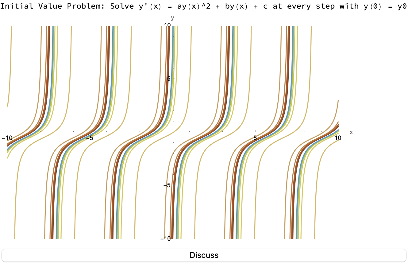
    "Initial Value Problem: Solve y'(x) = ay(x)^2 + by(x) + c at \
every step with y(0) = y0"],
   Show[plots[[All, 2]], PlotRange -> All, ImageSize -> Large],
   Button[
    "Discuss",
    CreateDialog[
     {
      TextCell[
       "Reflect on the impact of each parameter on the graph's \
shape."],
      DefaultButton[]}]]}],
 Initialization :> {a = 1, b = 1, c = 1}]

We need some effective communication in mathematics. Let's say we want to explain the Metropolis-Hastings algorithm, we've got all these candidate draws and want them to update, we want to know the acceptance rate as we converge with the Gibbs sampling. There's no pre-conditions for predicting what the Bayes Net is going to do. So if we want to describe the algorithm's steps and its role in sampling and data analysis, we could visualize the convergence of the MH algorithm and manipulate parameters to see their effects. All of these things foster a deeper understanding of the algorithm's behavior and applications. Historical context allows us to teach epidemiology, within the context of real-world problems where it is applied whether that's machine learning, physics, and/or "Transmission parameters estimated for Salmonella typhimurium in swine using susceptible-infectious-resistant models and a Bayesian approach.". It's really just a matter of finding human-specific cases of Salmonella, the values we got are specific to Salmonella typhimurium in swine. And that's definitely something that we can parse out, the population into the SIR model that we cherish, and strive to support mathematical discourse about our findings.

(*animatePlot :=*)
Manipulate[
 DynamicModule[{equations, solution, N},
  N = susceptible + infected + recovered;
  equations = {
    s'[t] == -transmissionRate*s[t]*i[t]/N,
    i'[t] == transmissionRate*s[t]*i[t]/N - recoveryRate*i[t],
    r'[t] == recoveryRate*i[t],
    s[0] == susceptible, i[0] == infected, r[0] == recovered};
  solution = NDSolve[equations, {s, i, r}, {t, 0, day}];
  Plot[
   Evaluate[{s[t], i[t], r[t]} /. solution],
   {t, 0, day},
   PlotLegends -> {"Susceptible", "Infected", "Recovered"},
   PlotStyle -> {RGBColor[1, 0, 1], RGBColor[1, 1, 0], 
     RGBColor[0, 1, 1]},
   AxesLabel -> {"Day", "Population"},
   PlotRange -> {0, N}]],
 {{day, 120, "Day"}, 1, 120, ControlType -> Animator},
 {disease, {"Salmonella", "Seasonal Flu", "Measles", "Smallpox"}, 
  ControlType -> PopupMenu},
 Dynamic[
  Switch[
    disease,
    "Salmonella",
    {transmissionRate = 0.33, recoveryRate = 0.14},
    "Seasonal Flu",
    {transmissionRate = 0.24, recoveryRate = 0.17},
    "Measles",
    {transmissionRate = 1.68, recoveryRate = 0.118},
    "Smallpox",
    {transmissionRate = 0.415, recoveryRate = 0.077}];,
  TrackedSymbols :> {disease} ],
 Dynamic@transmissionRate,
 Dynamic@recoveryRate,
 Initialization :> (
   susceptible = 500; infected = 10; recovered = 0;
   transmissionRate = 0.24; recoveryRate = 0.17;
   disease = "Salmonella"),
 ControlPlacement -> Left]
SetDirectory[NotebookDirectory[]];
Export["epidemic_simulation.gif", animatePlot, 
 "DisplayDurations" -> 0.1, "AnimationRepetitions" -> Infinity]

It's this forward-thinking approach that brings the old-fashioned, mathematics education and makes it more relatable and understandable. There's a place I know where historical context can make complex mathematical ideas more relatable and understandable. This is key to engaging students and fostering a positive learning environment, and with computational tools like the Wolfram Language we haven't been out of a definition for fundamental approaches to effective math teaching. Sometimes we want to know, how many practical applications are there of abstract mathematical theories? How can we provide more visuals? There are so many things that can be integrated with our approach, to chronologically explain the development of computation and computational thinking. I think for the field of mathematics education, placing an emphasis on slowing down the learning process might allow students to interact more comprehensively with the concept of mathematics, and discuss the kind of things that it provides. Taking a student-centric approach and integrating these computational tools, understanding the historic context and precedence for mathematics education..all of this stuff could serve as a model for educators seeking to make mathematics more accessible, engaging, and relevant to students.

I know it's the cherry blossom of metamathematics! What if you wanted to climb Mount. Fiji well I couldn't do it without your help.