The machinery that exists like clockwork and levers and all that kind of toroidal grid with diagonal connections stuff in which we can run a cellular automaton on it and then attempt to map the results to a 3D layout, these topological surfaces can serve as a starting point for experiments on different surfaces such as the Klein Bottle or Real Projective Plane by modifying how edges wrap around or how you choose to visualize the final graph. And I know the grid is topologically a torus. Forget the two-dimensional grid we can wrap the edges both horizontally and vertically to effectively construct the diagonal torus.
torusGrid[n_Integer, m_Integer] :=
  Module[{vertices, horizontalEdges, verticalEdges, diagonalEdges},
   vertices = Flatten[Table[{i, j}, {i, n}, {j, m}], 1];
   horizontalEdges =
    Flatten[Table[
      UndirectedEdge[{i, j}, {i, Mod[j, m] + 1}], {i, n}, {j, m}]];
   verticalEdges =
    Flatten[Table[
      UndirectedEdge[{i, j}, {Mod[i, n] + 1, j}], {i, n}, {j, m}]];
   diagonalEdges =
    Flatten[{Table[
       UndirectedEdge[{i, j}, {Mod[i, n] + 1, Mod[j, m] + 1}], {i,
        n}, {j, m}],
      Table[UndirectedEdge[{i, j}, {Mod[i, n] + 1,
         Mod[j - 2, m] + 1}], {i, n}, {j, m}]}];
   Graph[vertices,
    Union[horizontalEdges, verticalEdges, diagonalEdges]]];
GSRule[g_Graph, init_List, survival_List, growth_List] :=
  Module[{nbrs},
   nbrs = Total[init[[#]] & /@ AdjacencyList[g, #]] & /@ VertexList[g];
   Table[
    If[init[[i]] == 0, If[MemberQ[growth, nbrs[[i]]], 1, 0],
     If[MemberQ[survival, nbrs[[i]]], 1, 0]], {i,
     Length[VertexList[g]]}]];
GSIterate[g_Graph, init_List, survival_List, growth_List, t_Integer] :=
   Module[{history, currentState, nextState}, currentState = init;
   history = {currentState};
   Do[nextState = GSRule[g, currentState, survival, growth];
    AppendTo[history, nextState];
    currentState = nextState, {t}];
   history];
listToGraph3D[g_Graph, state_List] :=
  Module[{coords2D, coords3D, vertexStyles},
   coords2D = GraphEmbedding[g];
   coords3D = MapThread[Append[#1, 0.5*#2] &, {coords2D, state}];
   vertexStyles =
    Table[i -> If[state[[i]] == 1, Red, Blue], {i, Length[state]}];
   g];
static3DEnhanced[g_Graph, init_List, survival_List, growth_List,
   t_Integer] :=
  With[{evolution = GSIterate[g, init, survival, growth, t]},
   listToGraph3D[g, evolution[[1]]]];
Module[{g, initialState}, g = torusGrid[15, 15];
 initialState = RandomInteger[{0, 1}, VertexCount[g]];
 static3DEnhanced[g, initialState, {2, 3}, {3}, 30]]
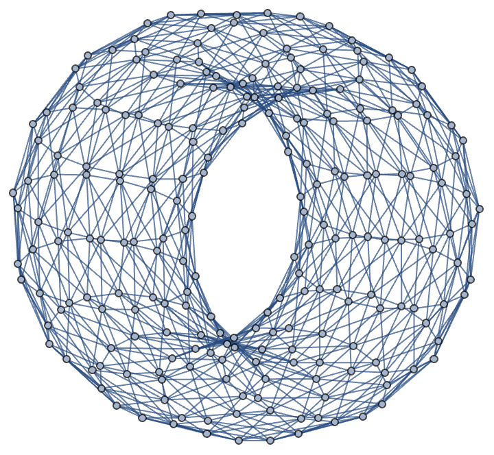
Excellent work, @Shuheng Li . And there are so many evolution paths for these initial conditions that we've built. Let's say we've got two neighboring columns of rules so to speak, we know they're geometrically nearby and that's important to our concept of forming images, whatever else. What is our map of smell, taste, and sound? Let's imagine we can detect the shape(s) of molecules because we can do that with nested molecules, and the order of operations doesn't matter. But what does matter is, I suppose, the compression of ideas...if we could uncompress our ideas and then project them back out we would see how we've got to find some balance between our ideas diverging to infinity and our squared ideas converging before reaching infinity, because we've been taking the concepts we care about like cellular automata..which are typically run on linear sequences or flat 2D grids..but it turns out that we can explore their behavior on surfaces with different topologies. It "doesn't care" that you can do this, because what we're doing is having the boat cross the genomic scene and Wolfram Alpha can figure out what is going on. In the end, it crushes the jar or the Klein Bottle of the tears in the different topologies we've got, because we don't want to learn too much and wander on and on with huge step sizes, but notation..we've done a lot to take the traditional mathematical notation like asterisks and there are famous examples, like the times sign and the dy/dX notation for Calculus, we could probably just keep walking over various surfaces including the Möbius Strip, the Sphere, the Torus, the Real Projective Plane, and the genus-2 surface just to "drop" a few using grids, and we're going to need to maintain our activation of these cellular automaton rules such as Rule 90 and Conway's Game of Life..and apply these rules to these surfaces represented as graphs.
torusGrid[n_Integer, m_Integer] := Module[
  {vertices, horizontalEdges, verticalEdges, g},
  vertices = Flatten[Table[{i, j}, {i, n}, {j, m}], 1];
  horizontalEdges = Flatten[
    Table[
     If[j == m,
      UndirectedEdge[{i, j}, {i, 1}],
      UndirectedEdge[{i, j}, {i, j + 1}]],
     {i, n},
     {j, m}
     ]
    ];
  verticalEdges = Flatten[
    Table[
     If[i == n,
      UndirectedEdge[{i, j}, {1, j}],
      UndirectedEdge[{i, j}, {i + 1, j}]],
     {i, n},
     {j, m}]];
  g = Graph[vertices, Join[horizontalEdges, verticalEdges]];
  Graph[g, VertexLabels -> "Name"]]
torus = torusGrid[10, 10]
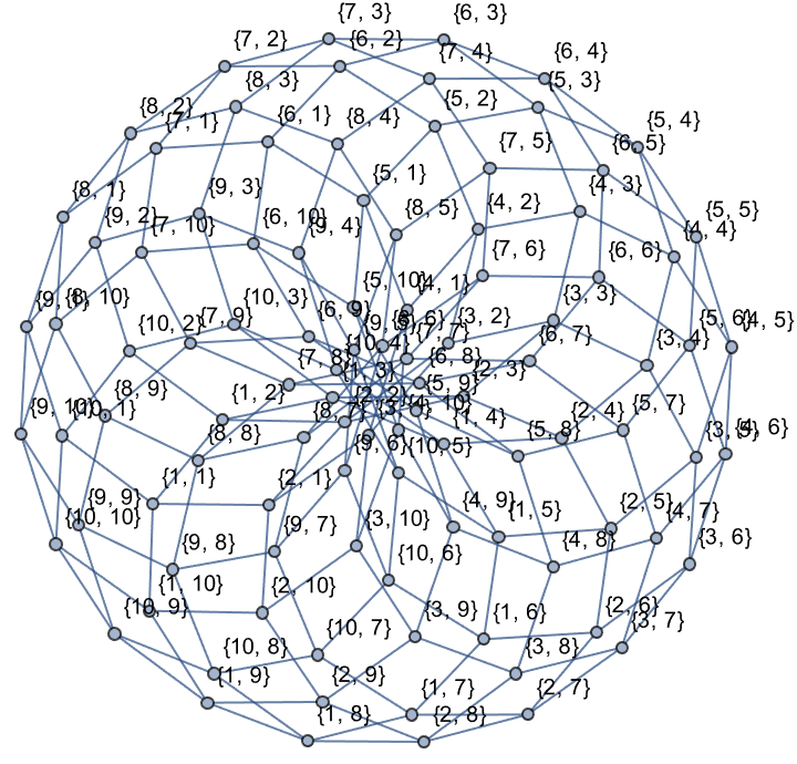
It's a question of, we do our thinking type of things to generate language..from these state transition diagrams, computed to analyze the behavior of CA on different surfaces, we bathe it in some volume of memory capacity and change your mood and the nerve cells, we can inherit the biases of an imbalanced dataset and trade it now for some variability, sensitivity that gives us some thing about, assuming that these artificial neural nets..what functions are easy to compute with neural nets and what are not? And the thing to understand is that digital computers are based on 1s and 0s, everything is discrete. Neural nets in their current construction are fundamentally continuous, and if you bash the thing, you train something to be slightly different..and that little extra change might really matter because you might just go above some threshold of some activation function, classification that can run in parallel, many bits make up an analog of some number, it's very similar to some analogy of the gradients of fluid mechanics, where there's this continuous velocity of fluid that's really made up of some molecules in some discrete form..but this question about the dimensionality of how neural network layers fill out the memory pool, just shows that when we want to compute these diagrams for larger grid sizes then there's an exponential increase in possible states.
diagonalGridGraph[n_Integer, m_Integer] := Module[
   {g, vertices},
   g = GridGraph[{n, m}];
   vertices = VertexList[g];
   NearestNeighborGraph[
    vertices,
    DistanceFunction -> ChessboardDistance
    ]
   ];
torusGrid[n_Integer, m_Integer] := Module[
   {g},
   g = diagonalGridGraph[n, m];
   EdgeAdd[g,
    Flatten[
     Table[
      {
       Mod[i, n, 1] \[UndirectedEdge] Mod[i + n - 1, n*m, n],
       Mod[i, n, 1] \[UndirectedEdge] Mod[i - n - 1, n*m, n]
       },
      {i, n*m}]]]];
torus = torusGrid[10, 10]
By 1.05, the cat is starting to have bizarre things sticking out of its head, the cat's amped up exploded network, could one take that network and continue training it, eventually that training would revert to what it's got before, skipping over the intermediate layers, and when we have all these gliders and lightweight spaceships..I wonder why, we will cut out all these transition diagrams and in short, we will highlight the quantitative and qualitative differences in nature.
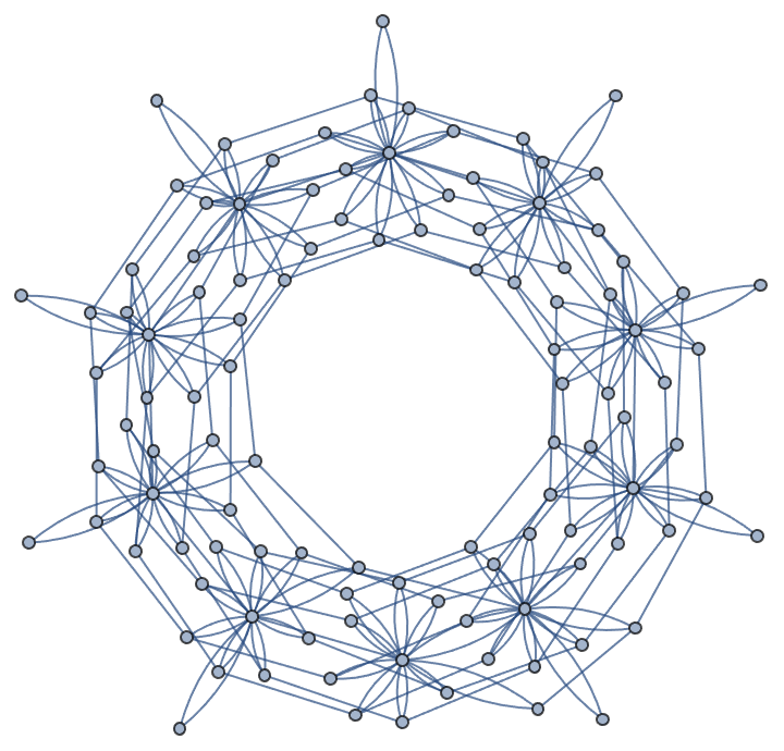
And we will save what we've got before and yes, unexpected things will happen. If you want computation in AIs to do the things that computation and AI can do, then you are signing up for computational irreducibility. The number of cycles and the behavior of gliders and spaceships can vanish, or it can explode depending on the topology of the surface. The degenerate optima that you might find in the divots across surfaces, and the self-propagating structures we did with Cellular Automata..these Cellular Automata are generalizable and there are all these things we can do in the natural world..wasn't built for us humans, and the niches that are naturally available...allow us to experiment with different transition rules sensitive to surface topology.
diagonalGridGraph[n_Integer, m_Integer] := With[
  {
   g = NearestNeighborGraph[GraphEmbedding@GridGraph[{n, m}],
     DistanceFunction -> (ChessboardDistance)]
   }, VertexReplace[g, # -> -VertexIndex[g, #] & /@ VertexList[g]]
  ]

torusGrid[n_Integer, m_Integer] := EdgeAdd[diagonalGridGraph[n, m],
   Union[
    {
        Range[1, n][[#]] -> Range[n*m - m + 1, n*m][[#]],
        Range[1, n][[#]] ->
         Range[n*m - n + 1, n*m][[Mod[# + 1, n, 1]]],
        Range[1, n][[#]] -> Range[n*m - n + 1, n*m][[Mod[# - 1, m, 1]]]
        } & /@ Range[1, m] //
     Flatten, {Array[m*# - m + 1 &, m][[#]] <-> Array[n*# &, m][[#]],
        Array[n*# - n + 1 &, m][[#]] <->
         Array[n*# &, m][[Mod[# + 1, m, 1]]],
        Array[n*# - n + 1 &, n][[#]] <->
         Array[n*# &, n*m][[Mod[# - 1, m, 1]]]} & /@ Range[1, m] //
     Flatten]
   ] // SimpleGraph

gliderLD[n_Integer, m_Integer, coordinate_List] :=
 ReplacePart[
  Array[0 &,
   n*m], {(coordinate[[2]] - 1)*n*m + coordinate[[1]] ->
    1, (coordinate[[2]] - 1)*n + coordinate[[1]] + n + 1 ->
    1, (coordinate[[1]] - 1)*n + coordinate[[2]] + 2 n - 1 ->
    1, (coordinate[[1]] - 1)*n + coordinate[[2]] + 2 n ->
    1, (coordinate[[1]] - 1)*n + coordinate[[2]] + 2 n + 1 -> 1}]

listToGraph[g_Graph, state_List] :=
 Graph[g,
  VertexStyle -> (If[
       state[[#]] == 1, # -> Black, # ->
        ColorData["CherryTones"] /@ {RandomReal[]}] & /@
     VertexList[g]), VertexSize -> 1]

neighborPopulation[g_Graph, init_List] :=
 Total[init[[#]] & /@ AdjacencyList[g, #]] & /@ VertexList[g]

GSRule[g_Graph, init_List, survival_List, growth_List] :=
 With[{N = neighborPopulation[g, init]},
  If[init[[#]] == 0, If[MemberQ[growth, N[[#]]] == False, 1, 0],
     If[MemberQ[survival, N[[#]]] == True, 1, 0]] & /@ VertexList[g]]

GSIterate[g_Graph, init_List, survival_List, growth_List, t_Integer] :=
  NestList[GSRule[g, #, survival, growth] &, init, t]

animate3D[g_Graph, init_List, survival_List, growth_List, t_Integer,
  speed_Integer : 1] :=
 With[{A =
    Graph[listToGraph[g, #], VertexCoordinates -> Automatic] & /@
     GSIterate[g, init, survival, growth, t]},
  Animate[A[[u]], {u, 1, t + 1, speed}]]

animate3D[torusGrid[15, 15],
 gliderLD[15, 15, {10, 10}], {2, 3, 4}, {3, 4}, 129, 1]
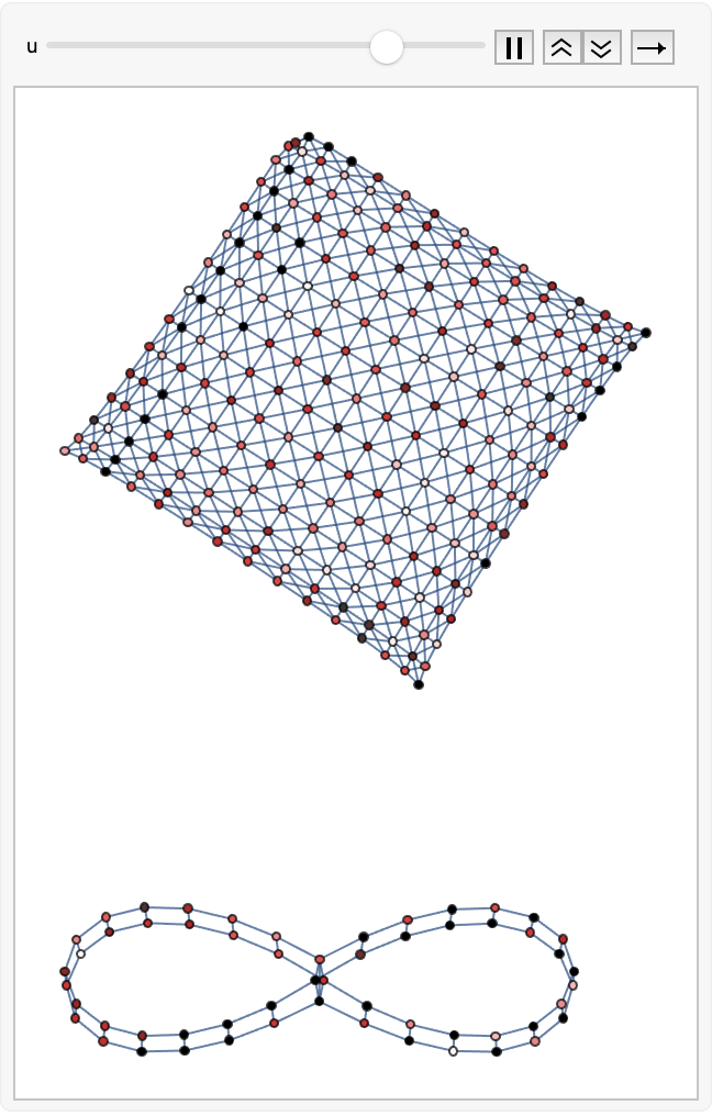
On these topological surfaces, we're going to be able to walk up the steps, we're going to be able to open the door. When you see me experiment with different transition rules..it might shed some light on how local rules interact with global surface properties..and explain comprehensively how we explore Cellular Automata behavior on various topological surfaces. It's a bad idea to read too much into our data and its derivatives, except when it's not. I must admit, we could choose to say enough is enough, we could just hangout and sit back..double the batch size doesn't double the batch accuracy..although we've got more graph unions of spaceship/glider transition diagrams across different surfaces, we still need to compute them to visualize how initial conditions evolve along different paths due to differing topology. It's easy to get clogged full of random colors. Things happen regularly, and so that's why we construct surface grids for our purposes; visualize Cellular Automata behavior and analyze transition diagrams.
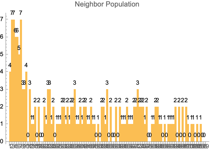
neighborPopulation[g_, init_] :=
  Total[init[[#]] & /@ AdjacencyList[g, #]] & /@ VertexList[g];
GSRule[g_, init_, survival_, growth_] :=
 With[{N = neighborPopulation[g, init]},
  If[init[[#]] == 0, If[MemberQ[growth, N[[#]]] == True, 1, 0],
     If[MemberQ[survival, N[[#]]] == True, 1, 0]] & /@ VertexList[g]]
GSIterate[g_, init_, survival_, growth_, t_] :=
 NestList[GSRule[g, #, survival, growth] &, init, t]
survival = {2, 3};
growth = {3};
iterations = 10;
initialState = RandomInteger[{0, 1}, VertexCount[torus]];
evolution =
  GSIterate[torus, initialState, survival, growth, iterations];
neighbors = neighborPopulation[torus, initialState];
BarChart[neighbors,
 ChartLabels -> Range[VertexCount[torus]],
 LabelingFunction -> Above,
 PlotLabel -> "Neighbor Population"
 ]
All these pockets of reducibility, all these devices jumping through computational reducibility. In our universe, we never get to fully transcend computational irreducibility. Pick another universe ...you can. It demonstrates the insights we get when we get more data, the best complexity increases and, whoops - nothing could possibly go wrong, everything is going to be alright. In some critical way, complexity doesn't compensate or compromise for the limitations in data of cellular automata, because the data is limited, and because there are so many permutations, when we reorganize the letters..the imputability gives us the importance of exploring periodicity, tessellated squares, and having fun just dropping everything and doing some implementations of the cellular automata that we haven't seen before, and yes, it really is our judgment of these local rules and global properties that give us all of the energy that we need to sufficiently traverse the stochastic gradient noise manner of surfaces, and if energy was sufficiently cheap, everything might as well fly. And there's a lot more room in 3-dimensional space than there is on Earth. Right now, I think that the topologies we've got are easy to explore, on the outer limits of our cellular automata perceptrons. And if we apply this reaction to this cellular automata, this final chain of surface topology and grid size and specified transition rules is a thing that's very generalizable and immune to small translations and transmutations of surface type and topology, that make wind turbines possible. And that's what makes Science and Technology so fun, like the forces that bind atoms together.