The extension idea for the Tropical Geometry and Newton Polytopes, it's important to remember that our original focus on converting classical algebraic polynomials into their tropical counterparts uses the MinPlus algebra and visualizes their contingent Newton Polytopes in two dimensions. I think last time I had put some three-dimensional visualizations of tropical hypersurfaces and now "hopefully" some interactive tools that allow us to dynamically investigate both quadratic and multivariate polynomials. And I say dynamic because, I think I had to tone down the full geometric beauty of tropicalization; I "had" some copyright issues with the multivariate polynomial in three variables because I was using the McDonald's logo to represent the three arches but it's true, we have these three cornerstones of the triangle. We have come into possession of all these snippets of three-variable polynomials p that are tropicalized using the MinPlus function. The tropical hypersurface then can be visualized via a 3D contour plot, while the corresponding Newton Polytope is constructed (and I don't really care whether it's yellow or some other non-copyrighted color), the extraction of exponent vectors and the 2-adic valuations of the coefficients. Thus I think what you'll see is that the function VisualizeTropicalGeometry that I am about to introduce..neatly arranges both plots side by side, offering a MORE IMMEDIATE visual insight into the "isomorphic" shape of the Newton Polytope as compared to the tropical hypersurface.
p = 8 x + 2 y + 5  z;
MinPlus[poly_] :=
  ReplaceAll[poly, {Plus -> Min, Times -> Plus, Power -> Times}];
TropicalHypersurface[poly_, variables_, range_] :=
  Module[{minPlusPoly, plot}, minPlusPoly = MinPlus[poly];
   plot =
    ContourPlot3D[minPlusPoly,
     Evaluate[
      Sequence @@ MapThread[{#1, -range, range} &, {variables}]],
     Mesh -> None, ContourStyle -> Opacity[0.5],
     ColorFunction -> Function[{x, y, z}, Hue[0.7 (x + y + z)]],
     PlotPoints -> 30, AxesLabel -> variables,
     PlotLabel -> "Tropical Hypersurface"];
   Return[plot];];
NewtonPolytope3D[poly_, variables_] :=
  Module[{tpoly, p, cs, P2 = poly},
   p = First /@ CoefficientRules[P2, variables];
   cs = IntegerExponent[#, 2] & /@
     Last /@ CoefficientRules[P2, variables];
   tpoly = Flatten /@ Transpose[{p, cs}];
   Show[ListPlot3D[tpoly, Mesh -> All, Axes -> True,
     PlotStyle -> {Yellow}, Filling -> Bottom],
    ListPointPlot3D[tpoly, PlotStyle -> {Red, PointSize[Large]}],
    AxesLabel -> Append[variables, "Valuation"],
    PlotLabel -> "Newton Polytope"]];
VisualizeTropicalGeometry[poly_, variables_, range_] :=
  Module[{tropicalPlot, newtonPlot},
   tropicalPlot = TropicalHypersurface[poly, variables, range];
   newtonPlot = NewtonPolytope3D[poly, variables];
   GraphicsRow[{tropicalPlot, newtonPlot}, ImageSize -> 600]];
VisualizeTropicalGeometry[p, {x, y, z}, 5]
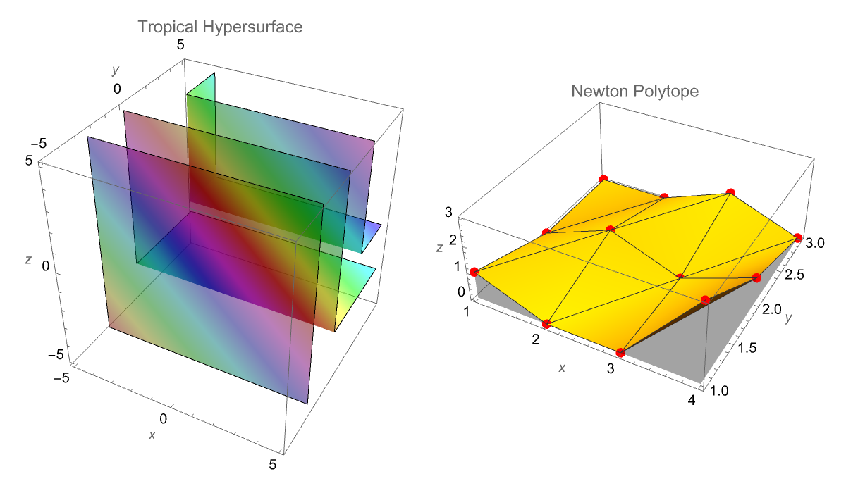
And that's how, if I put red dots all over it then it conveys the same message but without the reliance on the three-pronged approach that I had taken what with the tropicalization of the three-variable polynomial p using the MinPlus function. While, the corresponding Newton Polytope is the "combination" of the extraction of exponent vectors & the 2-adic valuations of the coefficients. For example, the Manipulate interface for a quadratic polynomial:
MinPlus[poly_] := poly /. {Plus -> Min, Times -> Plus, Power -> Times};
coord3D[poly_, variables_] :=
  Flatten /@
   Transpose[{First /@ CoefficientRules[poly, variables],
     IntegerExponent[#, 2] & /@
      Last /@ CoefficientRules[poly, variables]}];
NewtonPolytope[poly_, variables_] :=
  Module[{tpoly, p, cs},
   p = First /@ CoefficientRules[poly, variables];
   cs = IntegerExponent[#, 2] & /@
     Last /@ CoefficientRules[poly, variables];
   tpoly = Flatten /@ Transpose[{p, cs}];
   Show[ListPlot3D[tpoly, Mesh -> All, Axes -> True,
     PlotStyle -> Directive[Yellow, Opacity[0.5]], Filling -> Bottom,
     FillingStyle -> Opacity[0.3], PlotLabel -> "Newton Polytope",
     AxesLabel -> {"x", "y", "Valuation"}, ImageSize -> 300],
    ListPointPlot3D[tpoly, PlotStyle -> {Red, PointSize[0.02]}]]];
Manipulate[
 With[{poly = a x^2 + b y^2 + c x y + d x + e y + f},
  Row[{ContourPlot[MinPlus[poly], {x, -5, 5}, {y, -5, 5},
     ExclusionsStyle -> Black,
     PlotLabel -> Style["MinPlus Transformation", 14, Bold],
     ImageSize -> 200, Contours -> 20,
     ColorFunction -> "SolarColors"], NewtonPolytope[poly, {x, y}]},
   Center]],
 Style["Quadratic Polynomial Coefficients", Bold,
  12], {{a, 1, "x² coefficient"}, -10, 10, 1,
  Appearance -> "Labeled"}, {{b, 1, "y² coefficient"}, -10, 10, 1,
  Appearance -> "Labeled"}, {{c, 1, "xy coefficient"}, -10, 10, 1,
  Appearance -> "Labeled"}, {{d, 1, "x coefficient"}, -10, 10, 1,
  Appearance -> "Labeled"}, {{e, 1, "y coefficient"}, -10, 10, 1,
  Appearance -> "Labeled"}, {{f, 1, "Constant term"}, -10, 10, 1,
  Appearance -> "Labeled"}, ControlPlacement -> Left,
 TrackedSymbols :> {a, b, c, d, e, f}, Paneled -> False]
So it's really the contour plot representing the MinPlus (tropical transformation) and the 3D Newton Polytope update. You can think of it like these sliders, form the pendulum of the sensitivity of tropical structures to their coefficient values. In our eyes we can slide the xy coefficient left and right, and left again and then combine multiple predefined polynomials into a "unified" interface; TabView lets the user (us) switch between a custom polynomial mode and a selection of pre-stored examples. This dual approach enriches the exploration of tropical geometry by allowing side-to-side comparisons and rapid testing of diverse polynomials. By the way, that's the number of trees as a function of the number of nodes; that sort of mathematical polynomial concidence is useful; I would say that's been much more successful, applying this to the natural world. There's another case of this in archaeology where people say oh the height of the Great Pyramid divided by the size of the nose of the Sphynx is very close to π^2, that must have been significant. Nobody knew that at the time that the pyramids were being built. Early printing, 1500s and 1600s hiding messages in the weird numbers that would show up in places. There's a sort of tradition of that in the Kabbalah Jewish tradition in the Old Testament and, did the people who were writing this hide a secret message in the number of Hebrew characters here and there or is that a coincidence? That's always a difficult question, was that thing made for a different purpose or so on is that a problem? If you see a hexagon drawn in the sand, you can reasonably "assume" it was made for a purpose by an intelligence of some kind. There are wind-produced patterns in the sand that can be hexagons but it's just the wind. Unless you think of the wind as an intelligence, as you should it's certainly not an intelligence of the human kind. If you look at the North Pole of the planet Saturn, it's a giant storm that looks like a hexagon right there. So in Immanuel Kant's heuristic, was it made for a purpose or was it made by intelligence, Saturn was made by intelligence. It talks about the difficulty of measuring what's intelligence or what's a natural thing? Marconi and Tesla had noticed that if you just put a radio mask up there wasn't a lot of radio transmission going on in the world at that time if you were in a "yacht" going across the middle of the Atlantic you would hear all kinds of radio emissions; what were they? Tesla said they must be the Martians signaling Marconi didn't know what they were..but what they actually are..are particular magnetohydrodynamic effects, in the Earth's ionosphere. And, they are essentially a pure piece of nature but "yet", they make these woo wroo wroo sounds that are an effect of nature..whale sounds sound like emissions from the ionosphere. Can we tell what was for a purpose and what wasn't?

The structure underlying topical polynomials, whether for academic investigation or interdisciplinary applications in physics & economics, we open new vistas to "advance our understanding" of the combinatorial and geometric properties of polynomials. At the patent office for instance we could sort of fall through the real-time tropical geometry and show an unexpected landscape of 2-adic valuation int he formation of Newton Polytopes. The "key" ingredient in these transformations is in fact the extraction of the highest power of 2 that divides a given coefficient, also known as the 2-adic valuation which is a "fresh" way of replacing the classical coefficient with a numerological number, its "tropical weight". "For" a number n, the 2-adic valuation v_{2}(n) is computed in Mathematica by: valuation = IntegerExponent[n, 2]. For instance..and I shouldn't say for example..consider the polynomial p = 5 + 8x + 2y.
MinPlus[poly_] :=
ReplaceAll[poly, {Plus -> Min, Times -> Plus, Power -> Times}];
NewtonPolytope[poly_, variables_] :=
Module[{tpoly, p, cs},
p = First /@ CoefficientRules[poly, variables];
cs = IntegerExponent[#, 2] & /@
Last /@ CoefficientRules[poly, variables];
tpoly = Flatten /@ Transpose[{p, cs}];
Show[ListPlot3D[tpoly, Mesh -> All, Axes -> True,
PlotStyle -> Directive[Yellow, Opacity[0.6]], Filling -> Bottom,
BoundaryStyle -> Thick, PlotLabel -> "Newton Polytope",
ImageSize -> 300],
ListPointPlot3D[tpoly, PlotStyle -> {Red, PointSize[0.02]}]]];
coord3D[poly_, variables_] :=
Flatten /@
Transpose[{First /@ CoefficientRules[poly, variables],
IntegerExponent[#, 2] & /@
Last /@ CoefficientRules[poly, variables]}];
polyList = {{x^2 + y^2, {x, y}}, {5 x^3 + 3 y^2 + 7 x y, {x,
y}}, {4*x^2 + 2*x*y + y^2 + 3*x + 2*y + 1, {x, y}}, {16 x^2 +
6 x y + 7 y^2 + 7 x + 5 y + 2, {x, y}}, {8 x^3 +
6 x^2 y + 7 y^3 + 7 x^2 + 5 y^2 + 2 x + 2 y, {x,
y}}, {2*x^3 + 3*x^2*y + 4*x*y^2 + y^3 + x^2 + x*y + y^2 + x +
y + 1, {x, y}}, {10 x^4 + 5 x^3 y + 7 x^2 y^2 +
3 x y^3 + y^4 + 8 x^3 + 4 x^2 y + 2 x y^2 + y^3 +
5 x^2 + 7 x y + 3 y^2 + x + y, {x, y}}};
filteredPolyList = Select[polyList, Length[Last[#]] == 2 &];
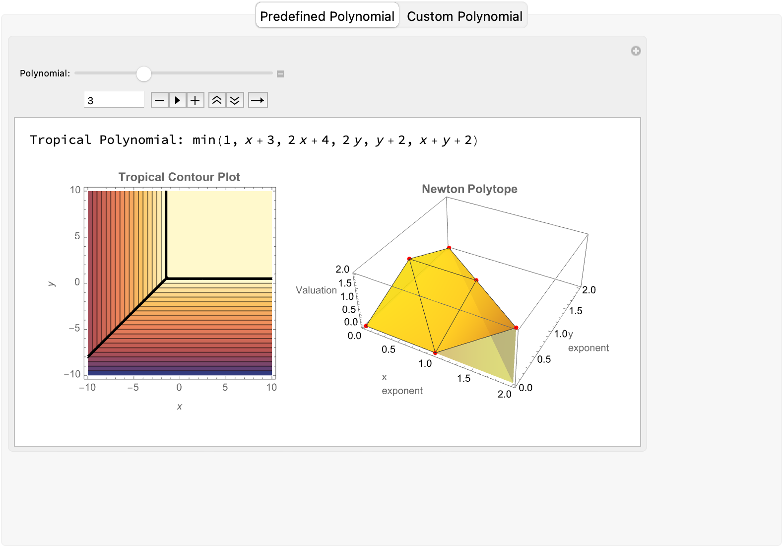
DynamicModule[{defaultTab = "Select a Tab"},
TabView[<|
"Predefined Polynomial" ->
Manipulate[
Module[{poly, vars, minPlusP, npPoints}, {poly, vars} =
filteredPolyList[[n]];
minPlusP = MinPlus[poly];
npPoints = coord3D[poly, vars];
Column[{Row[{"Tropical Polynomial: ",
TraditionalForm[minPlusP]}],
GraphicsRow[{ContourPlot[minPlusP, {x, -10, 10}, {y, -10, 10},
ExclusionsStyle -> Black,
PlotLabel -> Style["Tropical Contour Plot", 12, Bold],
ImageSize -> 222, FrameLabel -> {x, y}, Contours -> 20],
Show[ListPlot3D[npPoints, Mesh -> All, Axes -> True,
PlotStyle -> Directive[Yellow, Opacity[0.8]],
Filling -> Bottom,
PlotLabel -> Style["Newton Polytope", 12, Bold],
ImageSize -> 300,
AxesLabel -> {"x\nexponent", "y\nexponent", "Valuation"},
Boxed -> True, FillingStyle -> Opacity[0.3]],
ListPointPlot3D[npPoints,
PlotStyle -> {Red, PointSize[0.02]}]]},
ImageSize -> 600]}]], {{n, 1, "Polynomial:"}, 1,
Length[filteredPolyList], 1, Appearance -> "Open",
ControlPlacement -> Top}, TrackedSymbols :> {n}],
"Custom Polynomial" ->
Manipulate[
Module[{poly, minPlusPoly, npPlot},
poly = a x^2 + b x y + c y^2 + d x + e y + f;
minPlusPoly = MinPlus[poly];
npPlot = NewtonPolytope[poly, {x, y}];
Row[{ContourPlot[minPlusPoly, {x, -5, 5}, {y, -5, 5},
ExclusionsStyle -> None,
PlotLabel -> "MinPlus Transformation",
Background -> Transparent, Frame -> False, ImagePadding -> 5,
ImageSize -> 300], npPlot, TraditionalForm[poly]}]], {{a,
1}, -10, 10, 1, Appearance -> "Labeled"}, {{b, 1}, -10, 10, 1,
Appearance -> "Labeled"}, {{c, 1}, -10, 10, 1,
Appearance -> "Labeled"}, {{d, 1}, -10, 10, 1,
Appearance -> "Labeled"}, {{e, 1}, -10, 10, 1,
Appearance -> "Labeled"}, {{f, 1}, -10, 10, 1,
Appearance -> "Labeled"}, ControlPlacement -> Top,
AppearanceElements -> {"Slider"}, FrameMargins -> None]|>,
defaultTab]]
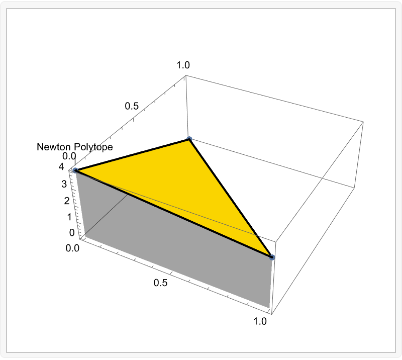
The 2-adic valuations are: v_{2}(8) = 3 (since 8 = 2^3), v_{2}(2) = 1 (since 2 = 2^{1}), v_{2}(5) = 0 (since 5 is not divisible by 2). These valuations are then used in forming the 3D coordinates of the Newton Polytope, it's the next thing that we collaborate on. The resulting coordinate list, for the polynomial p with respect to x and y, is {1, 0, 3, {0, 1, 1}, {0, 0, 0}}, which then forms the vertices of the Newton Polytope.

By swapping polynomial predefinitions with different inputs on that polynomial..the "Predefined Polynomial" mode encourages users--whether newcomers or veteran researchers--to experiment with different polynomial inputs as well as the resulting tropical structures. A selection of pre-stored examples switches "into" the custom polynomial mode, wherein the contour plot represents the MinPlus (tropical) transformation and the 3D Newton Polytope. You might call it a computational staircase to nowhere but this is a common sight, when we're looking at Stonehenge or something and ask was it set up this way because of the Equinox, or because Druid Xexteres decided what Stonehenge should look like. And sometimes you know in some of these cases when one says it's very accurately aligned so that the light falls on this stone at the time of the Equinox well, maybe they meant it to be the Equinox but they didn't know their astronomy well enough and so it's not aligned, it's very difficult to tell. Only a master could tell..
Laminar flow is when the fluid slides faster, when the fluid is going faster turbulence, is when it's making all these little eddies of air or water or whatever it's dealing with and there's this general cascade that happens, the eddies get ground down into smaller and smaller eddies and those eddies get cast away, a somewhat accurate universal law that the energy of a certain eddy is e^{5/3} law, the wave number is k^{-5/3} power, the reason for the gusting has to do with that kind of cascade of eddy sizes. So it's not completely sort of pure random because there's some sort of regularities from the size of the eddies' cascade and so on; when you look at the individual molecules you'll say they're pretty random; if you roll the clock back and work out the computation to where the molecules will be now. This phenomenon of computational irreducibility is that you can work out where these computations will be, these molecules for "practical purposes" you can't know where the molecules will be and you just have to "try" to say they seem random because you can't predict where they'll be. It's two-dimensional but we can make more plots, we can visualize a two-dimensional tropical curve in a ContourPlot of the tropicalized polynomial.
Manipulate[
 Show[
  ListPlot3D[
   coord3D[Round[c] 2 + 8 x + 5 y, {x, y}],
   Mesh -> None,
   Axes -> True,
   PlotStyle -> {Yellow},
   Filling -> Bottom,
   BoundaryStyle -> Thick,
   PlotLabels -> "Newton Polytope"],
  ListPointPlot3D[
   coord3D[Round[c] 2 + 8 x + 5 y, {x, y}]
   ]], {c, 1, 10}]
This precious article on the Newton Polytopes & those 3D coordinates, the co-efficients, the valuations, and most of all, an in-depth look at Tropical MinPlus algebra. Here, we have used the same polynomial p as above.
Maybe some other kind of operations... like the one with regard to grouping, distribution, and order of operands. Or to the highest prime of numbers like 3 or 5, also, with regard to the CoefficientRules is this good? Hard-code variables like x and y?
coord3D[poly_, variables_] :=
 Flatten /@
  Transpose[{First /@ CoefficientRules[poly, {x, y}],
    IntegerExponent[#, 2] & /@
     Last /@ CoefficientRules[poly, {x, y}]}]
Analyze polynomials? Using the MinPlus algebra which removes and mainly focuses on Newton Polytopes in the context of Tropical Geometry, don't say that combines algebraic geometry and combinatorics. Look at tropicalization, also known as the degeneration of algebraic varieties into tropical varieties. A multivariate polynomial is associated with integral polytopes and integral polytopes are associated with and can be used to study the polynomial's behavior. Remove duplicates, and explain the concept of MinPlus algebra and Tropical Semiring; a polynomial can be converted into a tropical polynomial consolidating this computationally universal aspect and approach of changing the operations of multiplication to addition and addition to minimum, moving on it's unprecedented. It's like the jacuzzi of vitality.
polyList = {
   {x^2 + y^2, {x, y}},
   {5 x^3 + 3 y^2 + 7 x y, {x, y}},
   {3 x^2 + 2 y z + z^2, {x, y, z}},
   {2 x^2 + 4 y^3 + x*y + 6, {x, y}},
   {4 x^2 + 6 x y + 7 y^2 + 5, {x, y}},
   {16 x^3 + 8 y^2 + 4 x*y + 2, {x, y}},
   {x^3 + y^3 + z^3 + 3 x y z, {x, y, z}},
   {x^4 + y^4 + x^2*y^2 + x + y + 1, {x, y}},
   {x^3 + z^3 + 2 x y z^2 + x y z + 1, {x, y, z}},
   {16 x^2 + 6 x y + 7 y^2 + 7 x + 5 y + 2, {x, y}},
   {x^3 + 2*x^2*y + 3*y^3 + x + y + 1, {x, y}},
   {4 x^3 + 2 y^2 + z^2 + 2 x*y*z + 1, {x, y, z}},
   {4*x^2 + 2*x*y + y^2 + 3*x + 2*y + 1, {x, y}},
   {x^4 + y^4 + z^4 + 4 x y z w + w^4, {x, y, z, w}},
   {3*x^2 + 5*x*y^2 + 7*y^3 + 2*x + y + 1, {x, y}},
   {2*x^2 + 3*y^2 + 4*z^2 + 5*x*y*z + 6, {x, y, z}},
   {8 x^3 + 6 x^2 y + 7 y^3 + 7 x^2 + 5 y^2 + 2 x + 2 y, {x, y}},
   {2*x^3 + 3*x^2*y + 4*x*y^2 + y^3 + x^2 + x*y + y^2 + x + y + 1, {x,
      y}},
   {x^3 + y^3 + z^3 + 3*x^2*y + 2*x*y*z + y^2*z + x + y + z + 1, {x,
     y, z}},
   {8 x^3 + 4 x^2 y + 6 y^2 z + 2 z^3 + 5 x^2 + 7 y^2 + 3 z^2 + x +
     y + z, {x, y, z}},
   {10 x^3 + 5 x^2 y + 7 y^2 z + 3 z^3 + 8 x^2 + 4 y^2 + 2 z^2 +
     5 x + 7 y + 3 z, {x, y, z}},
   {7*x^3 + 3*x*y + y^2 + 6*y + 9, {x, y}}, {3 x^2 + 6 y^2 + 2 z^2 +
     7 x + 3 y + 4, {x, y, z}},
   {10 x^4 + 5 x^3 y + 7 x^2 y^2 + 3 x y^3 + y^4 + 8 x^3 + 4 x^2 y +
     2 x y^2 + y^3 + 5 x^2 + 7 x y + 3 y^2 + x + y, {x, y}}};
NewtonPolytope[poly_, variables_, style_] :=
 Module[{tpoly, p, cs, P2 = poly},
  p = First /@ CoefficientRules[P2, variables];
  cs = IntegerExponent[#, 2] & /@
    Last /@ CoefficientRules[P2, variables];
  tpoly = Flatten /@ Transpose[{p, cs}];
  Show[ListPlot3D[tpoly, style, Mesh -> All, Axes -> True,
    Filling -> Bottom], ListPointPlot3D[tpoly]]]
commonStyle = {PlotStyle -> {Thickness[0.004], Blue},
   ColorFunction -> Function[{x, y, z}, Hue[1.0 z]], MeshStyle -> Red,
    ImageSize -> Large};
plots = Table[
   NewtonPolytope[First[i], Last[i], commonStyle], {i, polyList}];
GraphicsGrid[Partition[plots, 5], Frame -> None]
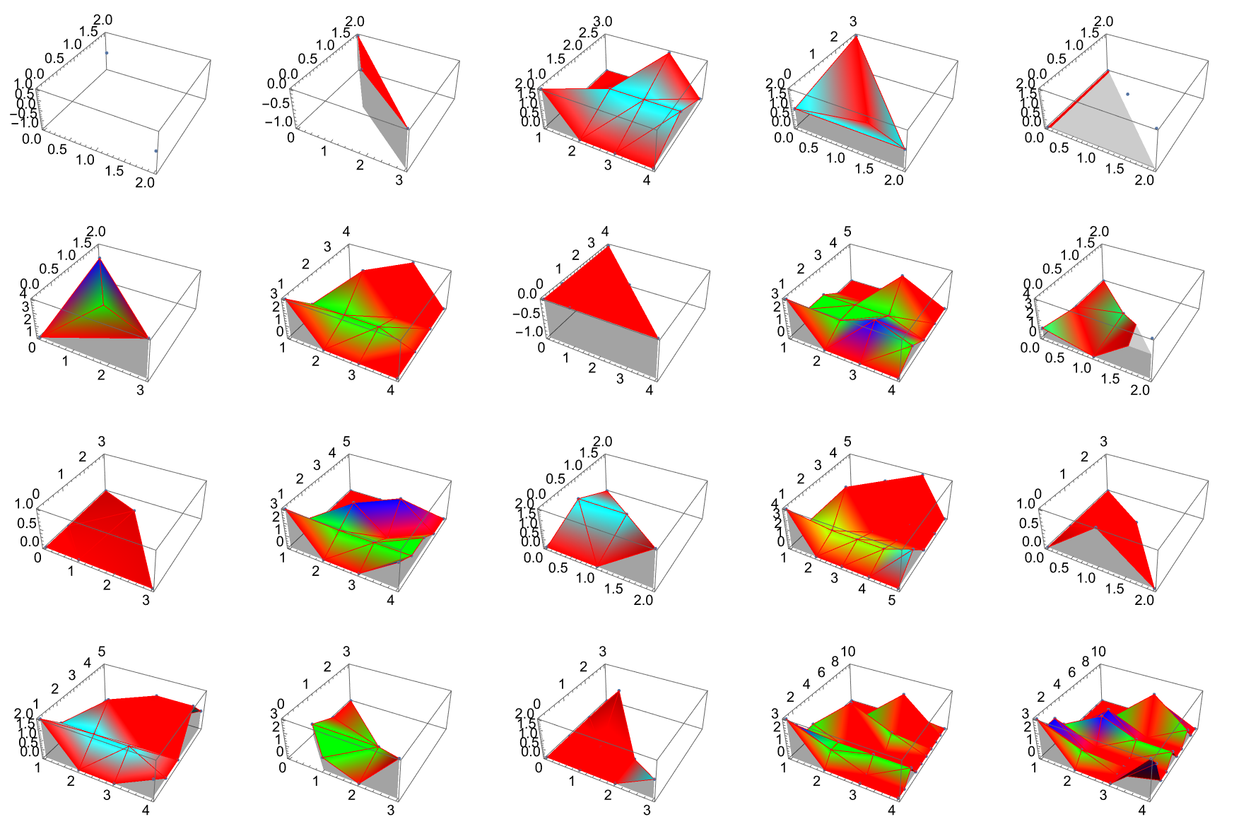
The transformation, give me a tutorial who does a deep dive into the topic of the 2-adic valuation, the technique used to find the right coefficients of a Tropical Polynomial like it's going out of style, precisely. For the 2-adic valuation for a number n that wouldn't be the same without being defined as the highest power of a prime p that divides n, no need to just provide some examples. Give me some code snippets to provide some grammatical interpretability and illustrate this universe concept. The splendid Newton Polytope of a given polynomial involves the people who labor and come out of the Earth just to get go form 3D coordinates, get exponent vectors and extract values from the valuation to form them in the first place, which springs forth the visualization of the Newton Polytope's opulence, in a three-dimensional plot.
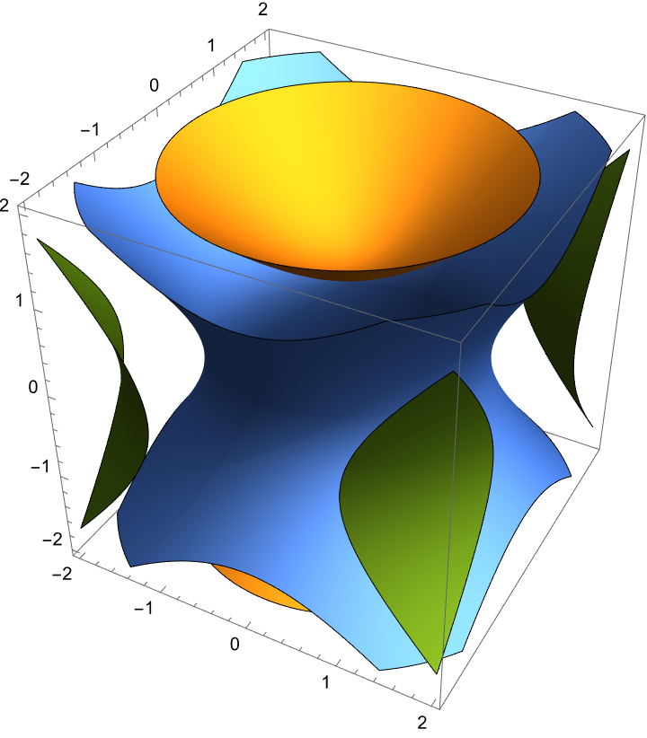
poly = x^2 + y^2 - z^2;
MinPlusPoly[poly_] :=
  ReplaceAll[poly, {Plus -> Min, Times -> Plus, Power -> Times}];
ContourPlot3D[MinPlusPoly[poly], {x, -2, 2}, {y, -2, 2}, {z, -2, 2},
 Mesh -> None]
What would happen if I tried to provide a substitution, or an in-depth exploration of Tropical Geometry and Newton Polytopes? That seems to target the audience who resides within the edifice of computational geometry and mathematical programming. @Afreen Naz reading is a joy, full of examples of mathematical software for geometric visualization and algebraic computation.
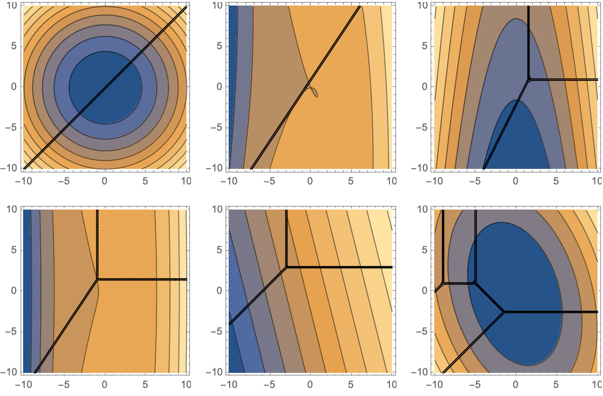
MinPlus[poly_] :=
  ReplaceAll[poly, {Plus -> Min, Times -> Plus, Power -> Times}];
polyList = {x^2 + y^2, 5 x^3 + 3 y^2 + 7 x y, x^2 + 2*y + 3,
   8 x^3 + 2 y^2 + 5, 8 x + 2 y + 5,
   16 x^2 + 6 x y + 7 y^2 + 7 x + 5 y + 2,
   8 x^2 + 2 x y + 3 y^2 + 4 x + 5 y + 6, 7 x^2 + 6 y^2 + 3 x y};
plots2D =
  Table[ContourPlot[MinPlus[poly], {x, -10, 10}, {y, -10, 10},
    ExclusionsStyle -> Black], {poly, Most[polyList]}];
poly3D = x^2 + y^2 - z^2;
plot3D =
  ContourPlot3D[MinPlus[poly3D], {x, -2, 2}, {y, -2, 2}, {z, -2, 2},
   Mesh -> None];
allPlots = Join[plots2D, {plot3D}];
GraphicsGrid[Partition[allPlots, 3]]
This new perspective has been a musical masterpiece in addressing enumerative problems. The application of this opportune discipline to physics & mathematics, hints at its interdisciplinary nature which is characteristically too big for the bottle of the study of particle motion using tropical shapes. It's more sort of incremental growth and there's certainly plenty of things that get done incrementally. And of course when you're dealing with incremental high growth there isn't a well-defined part you go on, you kind of have to invent things for yourself. What questions are worth asking?


