Hello. @Utkarsh Bajaj your hypergraph re-writing really shows these Turing Machines, the lambda calculus, the outputting of the functional register machine.
RMtoHypergraph[<|1 -> 0, 2 -> 1,
  3 -> 2|>, {{1, "-", 2, 4}, {3, "+", 3}, {2, "+", 2}}, 100]
The most precious thing about this is how you did it physically. We can actually see the register now.
RMtoHypergraph[<|1 -> 5, 3 -> 0,
  2 -> 3|>, {{1, "-", 2, 4}, {3, "+", 2}, {2, "+", 2}, {3, "-", 5,
   0}, {1, "+", 4}}, 10]
When you turn the tape into the hypergraph, that is our notion of computability and it's okay!
initialTapeToHypergraph[word_List] :=
Module[{x, y, z}, x = initialWordToHypergraph[word];
z = MinMax[
VertexList[
concatenategraphs[stateGraph[394], alphabetGraph[word[[2]]]]]];
y = MinMax[VertexList[x]];
Join[x, {{y, z + 1, z + 10}, {z + 1, z + 2, z + 3, z + 8}}]]
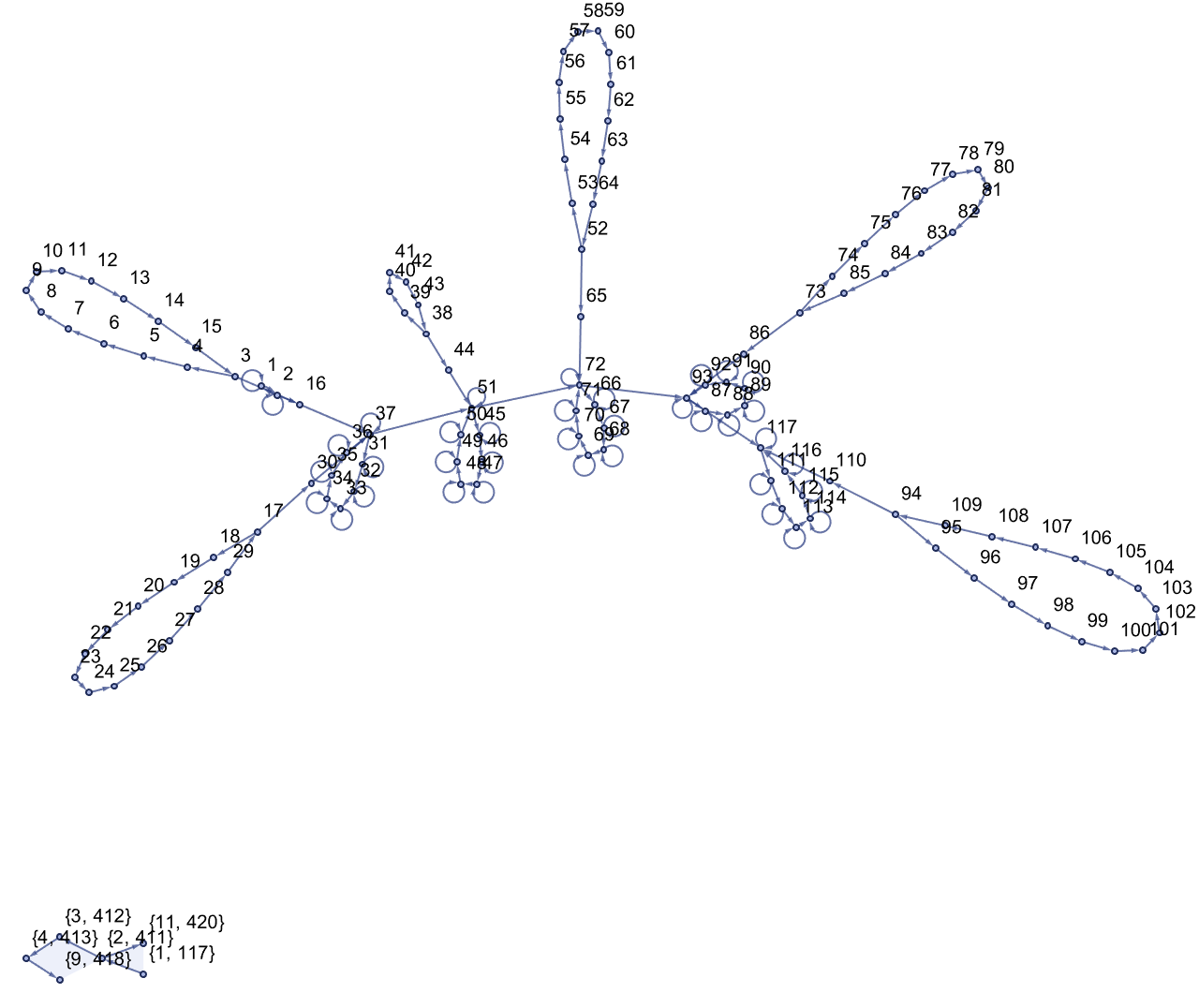
inputList = {12, 12, 5, 12, 12, 15};
ResourceFunction["WolframModelPlot"][
initialTapeToHypergraph[inputList], VertexLabels -> Automatic]
Hypergraph re-writing systems reminds me of the fractional dimensional nature of concurrent programming, this is the boundless conversion of finite state machines.
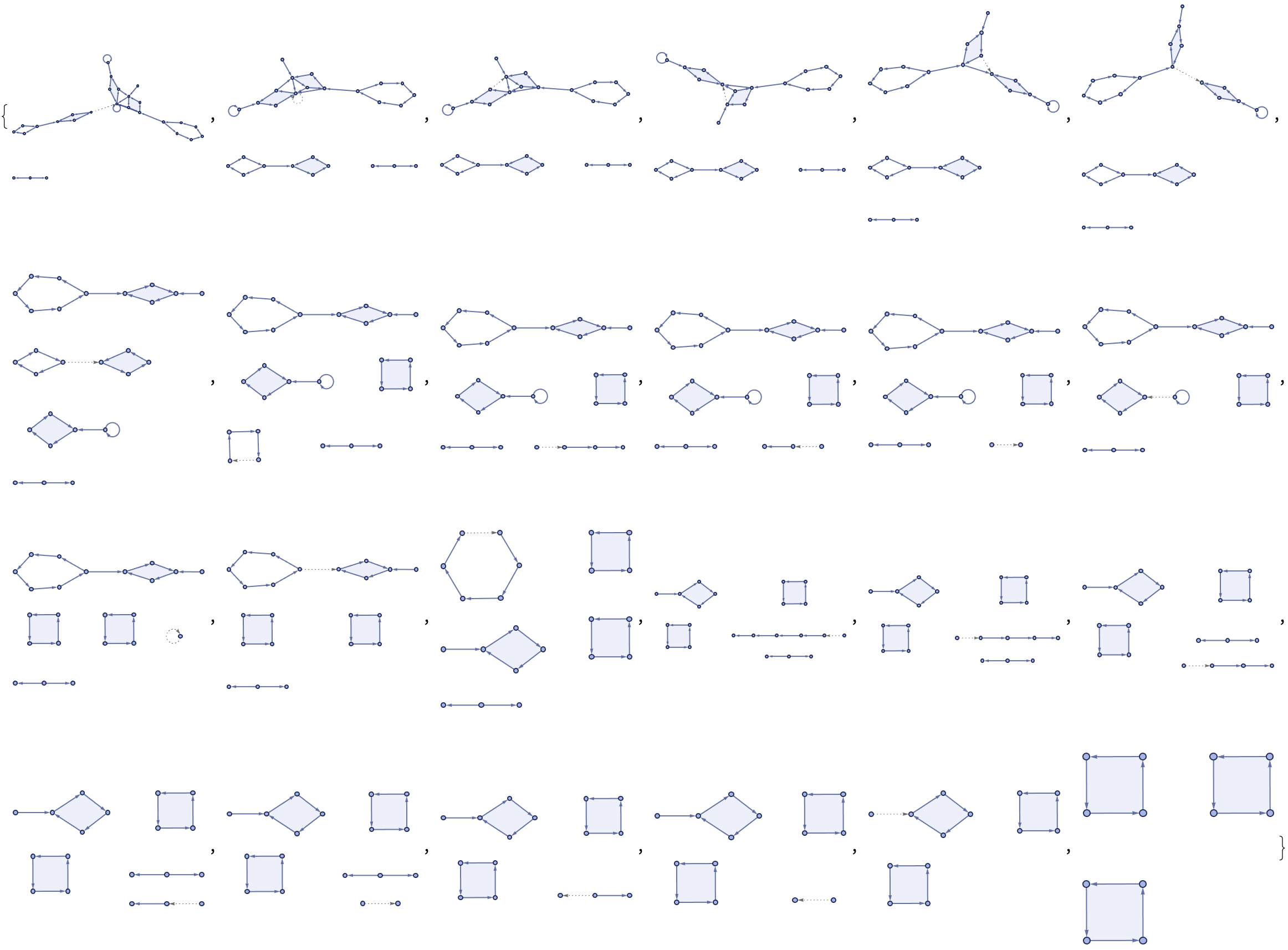
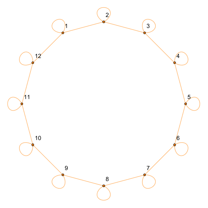
stateGraph[n_] :=
 Join[Table[{i, i + 2}, {i, 1, n}], Table[{i, i + 1}, {i, 1, n}]]
ResourceFunction["WolframModelPlot"][#, VertexLabels -> Automatic] & /@
  Table[stateGraph[n], {n, 1, 16}]
Can you imagine that, symbols in the alphabet and then graphs for each state?
DFAtoHypergraph[rules_List, word_List] :=
 ResourceFunction["WolframModel"][
  Table[DFARule[i], {i,
    Map[Join[#[[1]], #[[2]]] &, (rules /. Rule -> List)]}],
  initialWordToHypergraph[word], Length[word], "EventsStatesPlotsList"]

DFAtoHypergraph[{{0, 0} -> {1}, {0, 1} -> {0}, {1, 0} -> {0}, {1,
    1} -> {1}}, {1, 0}]
Concurrently because the process of converting NFAs to hypergraph rewriting systems is computationally expensive, and you could call it that because it's an area of future research. But you're providing this general reference frame.
alphabetGraphHelper[n_, m_ : 1] := If[n == 0,
{{1, 1}, {1, 2}},
If[n == 1,
{{1, 2}, {2, 1}},
Module[{x},
x = Last[#][[1]] &[alphabetGraphHelper[n - 1, Mod[m, n] + 1]];
Join[
Drop[#, -1],
{{x, x + 1},
{x + 1, 1},
{n + 2, n + 2 + m}}
] &[alphabetGraphHelper[n - 1, m + 1]
]
]
]
]
alphabetGraph[n_, m_] := If[n == 0,
{{1, 1}, {1, 2}},
Append[
alphabetGraphHelper[n, m],
{1, n + 2 + m}
]]
stateGraph[n_, m_] := Join[
Table[
{i, i},
{i, 1, n + 3 + m}
],
Table[
{i, i + 1},
{i, 1, n + 3 + m - 1}
], {{n + 3 + m, 1}}
]
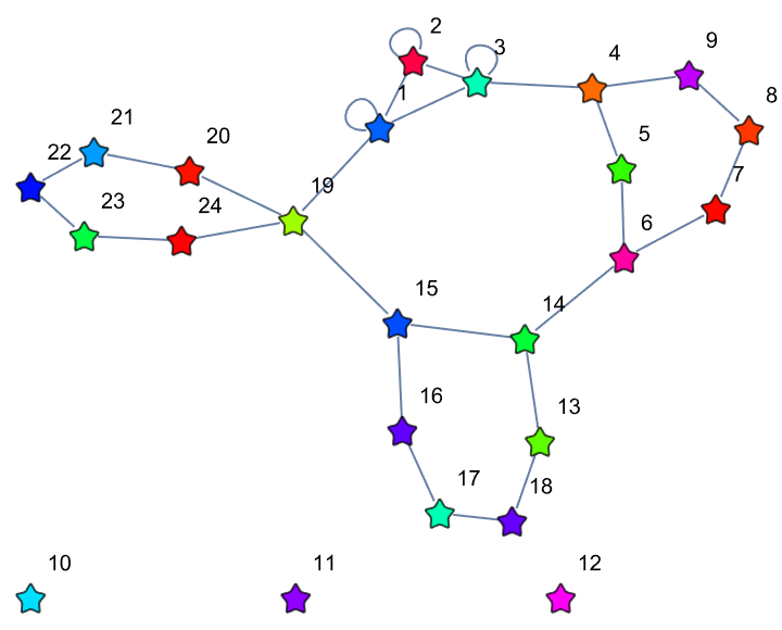
alphabetGraphData = alphabetGraph[4, 3];
alphabetGraphPlot = Graph[
alphabetGraphData,
VertexLabels -> Automatic,
VertexSize -> 0.05,
VertexStyle -> RGBColor[1, 0.5, 1],
EdgeStyle -> Directive[
Opacity[0.5],
ColorData[93, 1]
],
EdgeLabels -> Automatic,
EdgeLabelStyle -> Directive[
RGBColor[0.5, 0, 0.5],
Bold,
12,
Background -> White
]
]
stateGraphPlot = Graph[
stateGraph[5, 4],
VertexLabels -> Automatic,
VertexSize -> 0.05,
VertexStyle -> Orange,
EdgeStyle -> Directive[
Opacity[0.5],
RGBColor[1, 0.5, 0]
]
]
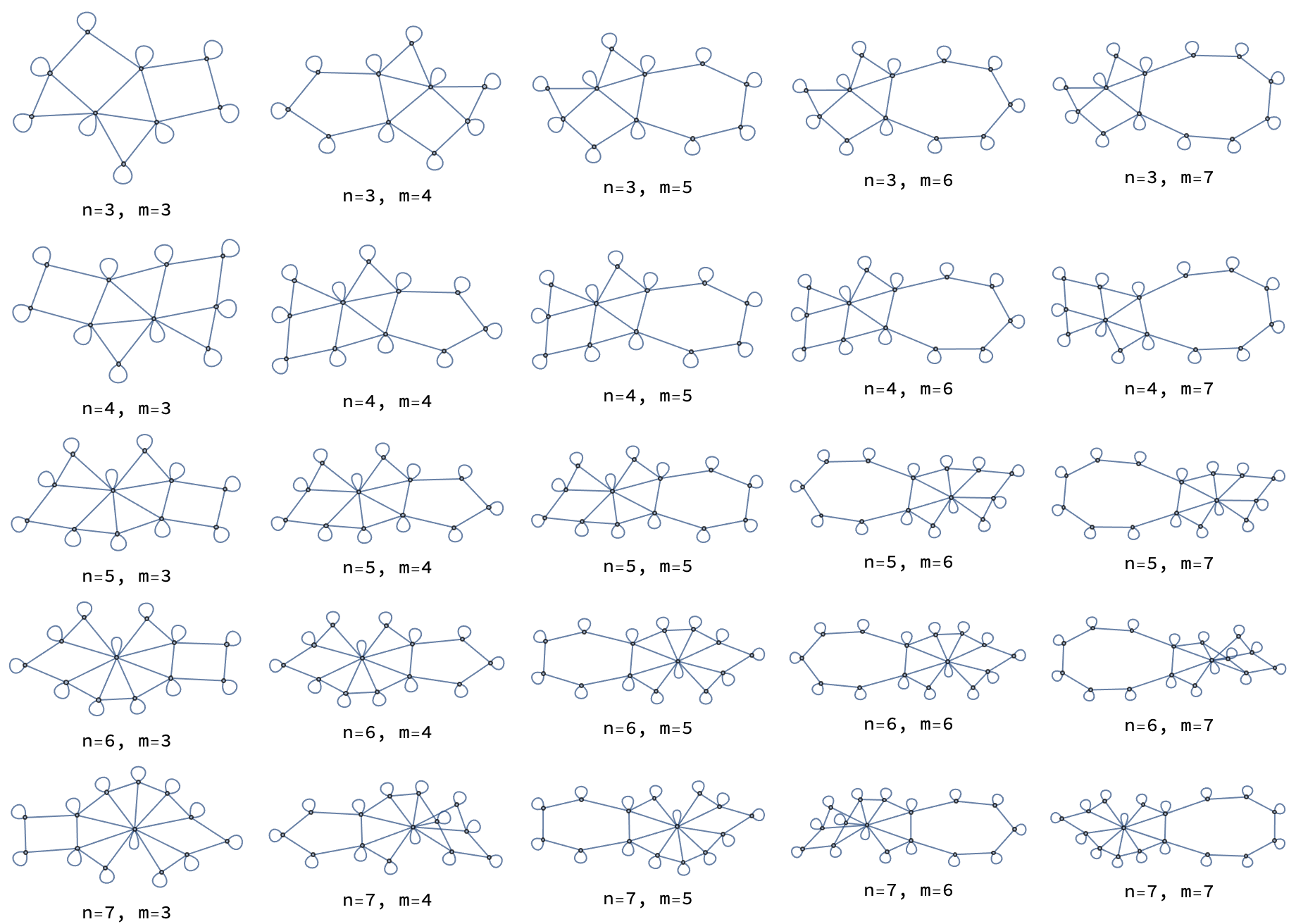
Grid[Table[Labeled[GraphUnion[
alphabetGraph[n, m],
stateGraph[n, m]
],
Row[{"n=", n, ", m=", m}]
], {n, 3, 7}, {m, 3, 7}]]
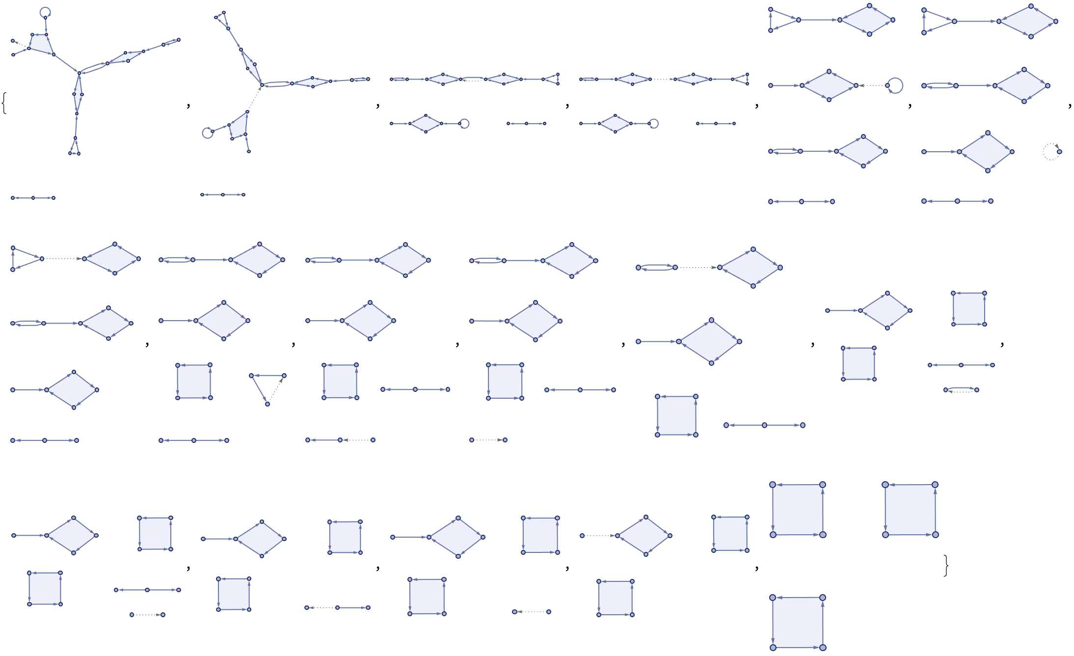
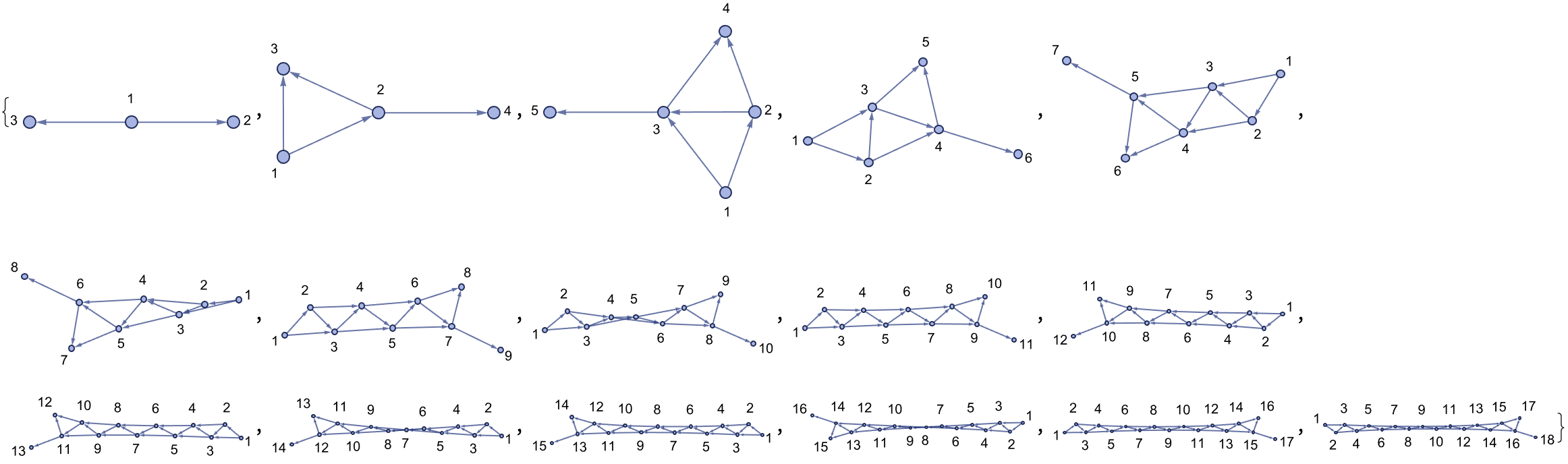
On the resulting substitution-based hypergraph re-writing system you're doing this magical data constructor.
These graphs have been cohesive joining your equivalence classes, which made the underlying abstract re-writing system happen.
JoinGraphs[g1_, g2_, state_] := Module[
{n},
n = Length[g1];
Join[g1,
{{Floor[n/2], n + 1}},
g2 + n,
{{Floor[n/2] + n, state}}
]];
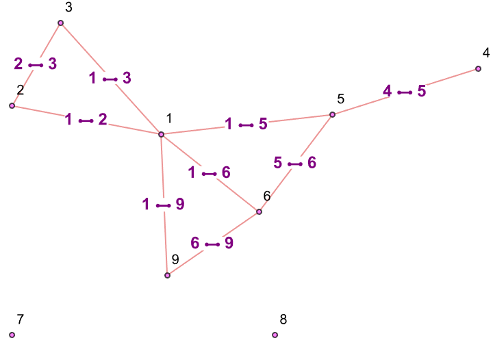
\[Chi] = JoinGraphs[\[Chi]2[5], \[Chi]3[5, 2], 1];
Graph[\[Chi],
VertexLabels -> Automatic,
VertexStyle ->
Thread[VertexList[\[Chi]] ->
Hue /@ RandomReal[{0, 1}, VertexCount[\[Chi]]]],
VertexSize -> Large,
VertexShapeFunction -> "ConcavePentagon"
]
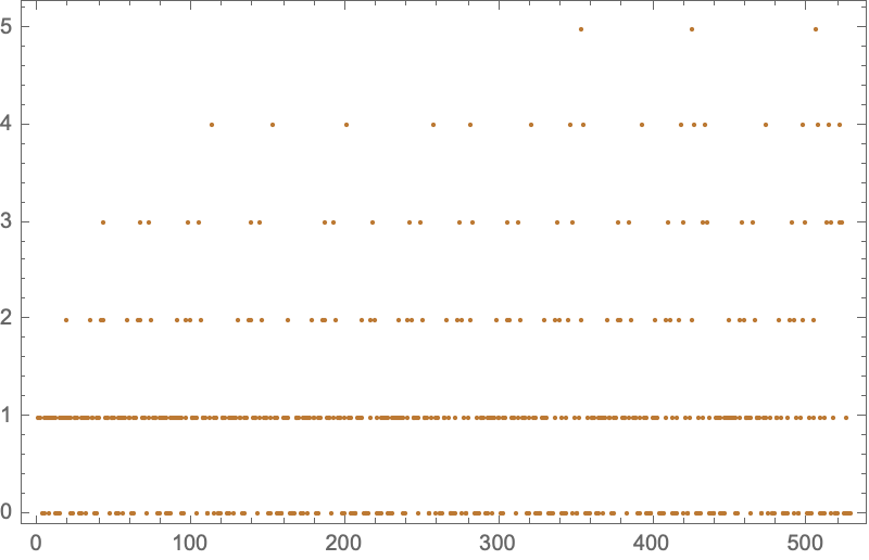
That was fantastic how you did the Faux Racket programming language into a hypergraph re-writing system using the operator notation, violating causal invariance.
initialTape = {1, 0, 1, 0, 1};
rulesTraditional = {{1, 0} -> {2, 1, 1}, {1, 1} -> {1, 1,
1}, {1, _} -> {5, _, 1}, {2, 0} -> {2, 0, 1}, {2, 1} -> {3,
0, -1}, {2, _} -> {3, 0, -1}, {3, 1} -> {4, 0, -1}, {4, _} -> {1,
0, 1}};
turingProgression =
Table[TuringMachine[rulesTraditional, {1, initialTape}, n], {n, 0,
10}];
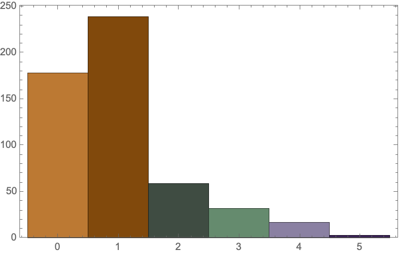
flattenedData = Flatten[turingProgression, \[Infinity]];
ListPlot[flattenedData, PlotStyle -> ColorData[41][10], Frame -> True,
ImageSize -> 400]
Histogram[flattenedData, Frame -> True, ImageSize -> 400,
ChartStyle -> ColorData[41]]
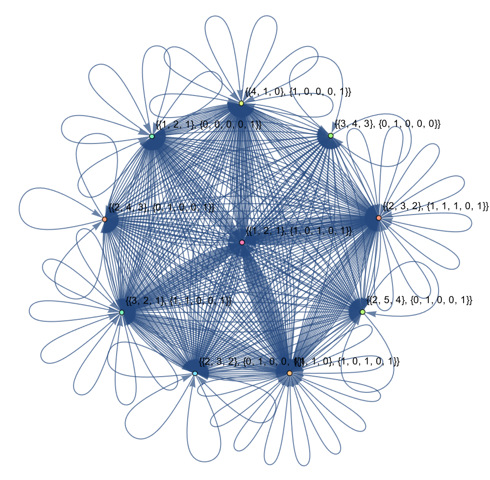
edges = Flatten[
Thread[Rule @@@ Tuples[{#, #2}]] & @@@
Partition[turingProgression, 2, 1], 1];
Graph[edges, VertexLabels -> "Name", VertexSize -> 0.05,
ImageSize -> 500,
VertexStyle ->
Thread[# -> Hue[RandomReal[], 0.5, 1] & /@
Flatten[turingProgression, 1]]]
The fundamental components that make up the Turing machine mean that there are a limited number of components, we just need to know the rules of those components, and one could say everything about how the computational universe works.