How did you know your 2d grid was going to just come up and with no explanation?
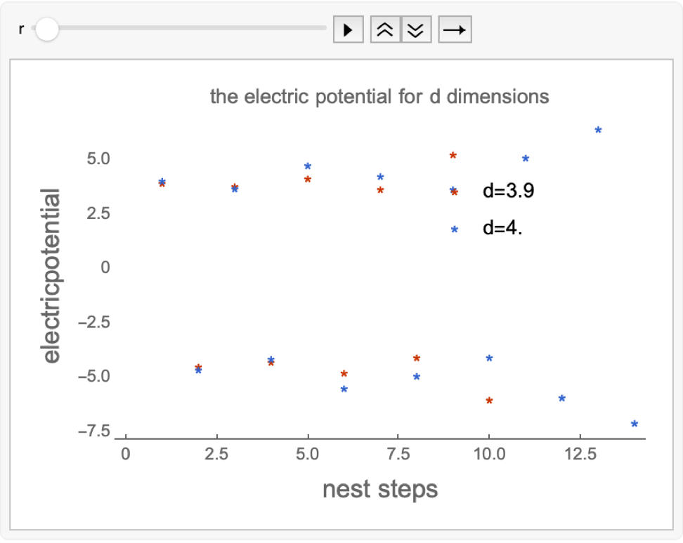
Subscript[electricpotential, r_][d_] :=
 Log[Gamma[(d/2) - 1]/(4*\[Pi]^(d/2))*1/r^(d - 2)]
Animate[ListPlot[
  {NestList[Subscript[electricpotential, r], 3.9, 1231],
   NestList[Subscript[electricpotential, r], 4, 1231]},
  PlotMarkers -> "*",
  PlotLegends -> Placed[{"d=3.9", StringJoin["d=4.", ""]}, {0.7, 0.7}],
  PlotTheme -> "Web",
  FrameLabel -> {Style["nest steps", 15],
    Style["electricpotential", 15]},
  PlotLabel -> "the electric potential for d dimensions"
  ],
 {
  {r, 1.64},
  1.64,
  1.7
  }
 ]
Sanjib many thanks for all this feedback, suggestions, support you guys are all rockstars. The point charge q finds electric field strength. The point charge q is kept colored black, and they are kept at a finite distance from each other. Is electromagnetic potential oscillatory? How do you get exact vertex weight?