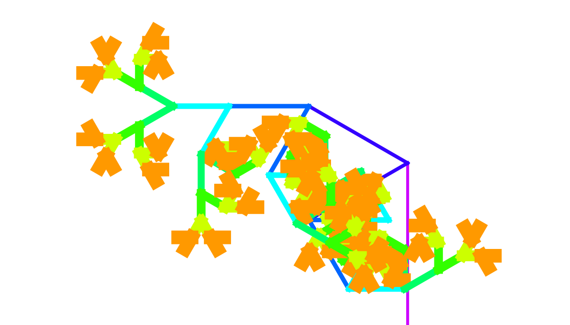
I think the tree data structure itself, the children can remain unevaluated until needed. The function ConsTree builds a finite tree up to a "specified" depth using a branch-generation rule. The three different rules are binary (produces two child branches at fixed angles), ternary (produces three branches with one continuing straight), random (randomly selects between two or three branches with slight variations).
SetAttributes[ConsTree, HoldRest];
Clear[GenerateFractalTree];
GenerateFractalTree[f_, initial_, 0] := ConsTree[initial, {}];
GenerateFractalTree[f_, initial_, d_Integer?Positive] :=
  ConsTree[initial,
   GenerateFractalTree[f, #, d - 1] & /@ f[initial]];
angleDelta = 30  Degree;
lengthFactor = 0.7;
binaryFractalRule[{len_, theta_}] := {{len*lengthFactor,
    theta + angleDelta}, {len*lengthFactor, theta - angleDelta}};
ternaryFractalRule[{len_, theta_}] := {{len*lengthFactor,
    theta + angleDelta}, {len*lengthFactor, theta}, {len*lengthFactor,
     theta - angleDelta}};
randomFractalRule[{len_, theta_}] :=
  Module[{numBranches, angleVariations},
   numBranches = RandomChoice[{2, 3}];
   angleVariations =
    If[numBranches ===
      2, {theta + RandomReal[{angleDelta/2, angleDelta}],
      theta - RandomReal[{angleDelta/2, angleDelta}]}, {theta +
       RandomReal[{angleDelta/2, angleDelta}], theta,
      theta - RandomReal[{angleDelta/2, angleDelta}]}];
   Map[{len*lengthFactor, #} &, angleVariations]];
treeType = "Binary";
branchRule =
  Switch[treeType, "Binary", binaryFractalRule, "Ternary",
   ternaryFractalRule, "Random", randomFractalRule, _,
   binaryFractalRule];
fractalDepth = 8;
fractalTree =
  GenerateFractalTree[branchRule, {1.0, Pi/2}, fractalDepth];
Clear[treeToLines];
treeToLines[ConsTree[node_, children_], startPos_ : {0, 0},
   startAngle_ : 0, depth_Integer?NonNegative] :=
  Module[{currentAngle, endPos, branchLine, childLines},
   If[depth == 0, Return[{}]];
   currentAngle = startAngle + node[[2]];
   endPos =
    startPos + node[[1]]*{Cos[currentAngle], Sin[currentAngle]};
   branchLine = {Thickness[0.03*(0.8^depth)], Hue[0.1*depth],
     Line[{startPos, endPos}]};
   childLines =
    Flatten[treeToLines[#, endPos, currentAngle, depth - 1] & /@
      ReleaseHold[children], 1];
   Prepend[childLines, branchLine]];
Graphics[treeToLines[fractalTree, {0, 0}, 0, fractalDepth],
 PlotRange -> {{-2.5, 1}, {0, 2}}, ImageSize -> Large]
Preventing infinite loops and ensuring that operations on self referential structures are meaningful and computationally effective, shows us how to create an infinite series of powers of two, generating sequences based on rules, and constructing infinite trees based on a pattern or rule. What is the algorithmic complexity of operations on the structures, are they in line with expectations for linked lists? There is a fine line between optimizing the code in terms of efficiency and runtime complexity. The practicality of operating on self referential expressions, and the applications of the data structures are the foundation of creativity. Our understanding of the potential and limitations of expressions that reference themselves and the ConsList and ConsTree, introduce the core question of whether or not we can effectively operate on self referential expressions. What are the "benefits" of constructing this framework? We are going to create some modified "versions" of the List and Tree structures that support operations on infinite, self referential objects.
SetAttributes[ConsList, HoldRest]
SetAttributes[ConsTree, HoldRest]
InfiniteSteps[head_, ID_, step_] :=
 ConsList[ID, InfiniteSteps[head, head @@ {ID, step}, step]]
Blockchain[initialBlock_] := NestConsList[BlockHash, initialBlock]
BlockHash[block_] := Hash[block, "SHA256"]
CoefficientOfRestitution[v_, e_] := -e*v
SimulateBounce[height_, e_] :=
 ConsList[height,
  If[height > 0.01,
   SimulateBounce[CoefficientOfRestitution[Sqrt[2*9.81*height], e],
    e], "Rest"]]
PrerequisiteTree[course_] :=
 ConsTree[course, PrerequisiteTree /@ Prerequisites[course]]
Prerequisites[course_] :=
 Switch[course, "Calculus", {"Algebra", "Geometry"}, "Algebra", {},
  "Geometry", {}, _, {"Algebra"}]
DisplayTreeLevels[tree_ConsTree, n_] := RootTree[tree, n]
steps = InfiniteSteps[Plus, 1, 1];
chain = Blockchain["Genesis Block"];
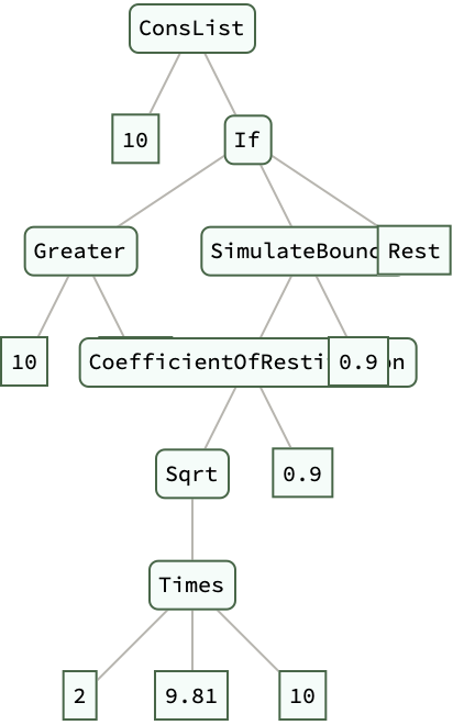
bounceSimulation = SimulateBounce[10, 0.9] // ExpressionTree
educationTree = PrerequisiteTree["Calculus"];
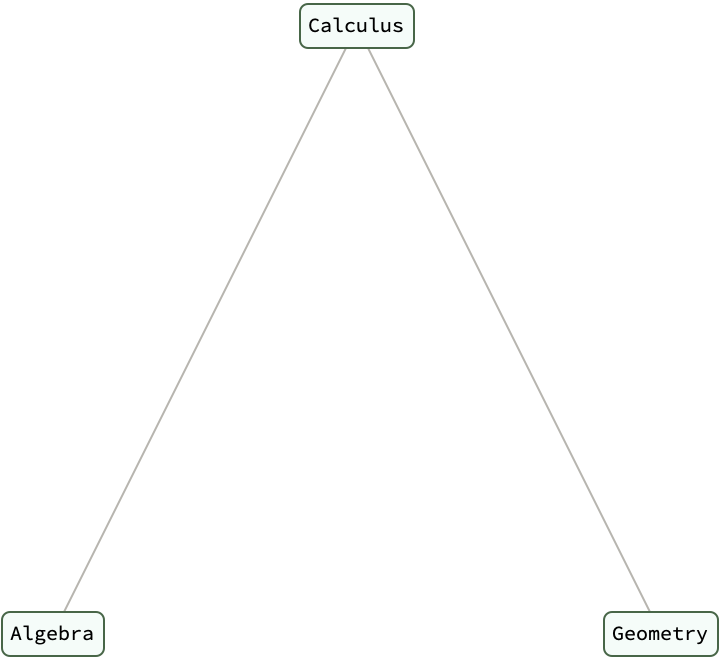
DisplayTreeLevels[educationTree, 3]
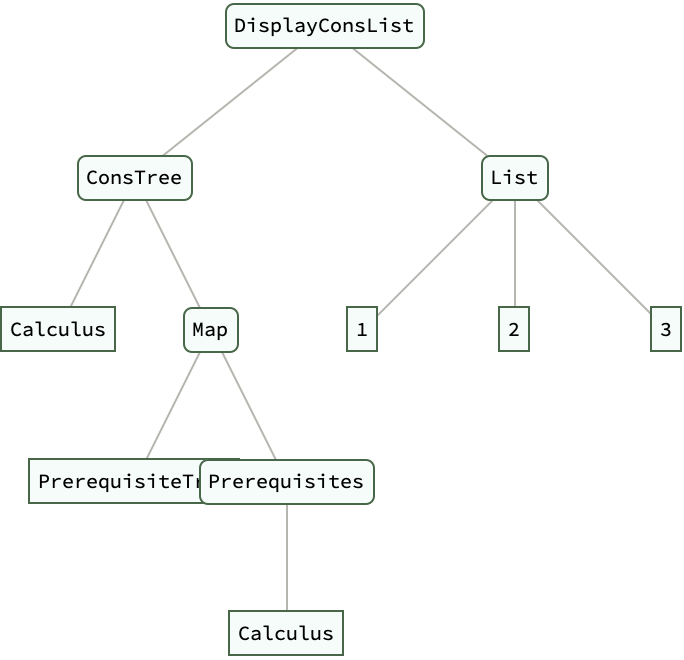
DisplayConsList[educationTree, {1, 2, 3}] // ExpressionTree
Ah, the framework for self-referential data structures. The University of Patras, that's a ConsList and ConsTree. We just screech and squeal and we had had to explore Lisp, algorithmic complexity. The motivations behind this project, the concept of lazy evaluation and the Lisp-like nature of the structures created, the collaborative spirit of the Wolfram method for exploring new ideas and refining computational methods. That is how the complexity of operations on the new data structures match up with the expected behavior of linked lists. That is how the Fibonacci sequence illuminates the practicality of operating on self referential expressions and the applications of graph theory principles. The ConsList and ConsTree data structure initialization is well worth the wait.
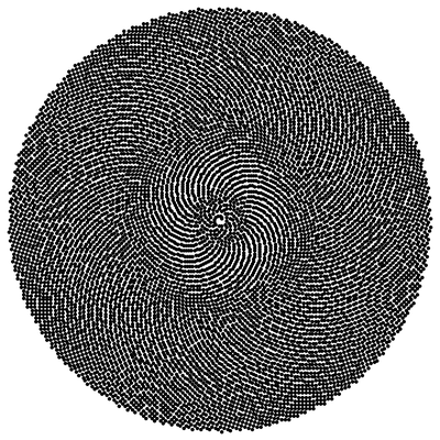
Take[InputSequence[#1 + #2 &, {# - 1, # - 2} &, {1, 1}], 30]
fib = %[[30]]/%[[29]]

Graphics[
 Point[Table[
   Sqrt[n] {Cos[0.1 Pi n fib], Sin[0.1 Pi n fib]}, {n, 10000}]]]
Which of these expressions are worth creating a framework for? It took me decades to get the possibility of operating on self-referential expressions. Sure x = {x, x} and the kernel prevents infinite evaluation by applying Hold to the expression. @Athina Kyriazi as for the "usefulness" of self-referential expressions, are they meaningful if they can solve problems? Are these ConsList and ConsTree introduced as self-referential types so just we can find something akin to the infinite list, while ConsTree resembles an infinite tree structure? What does it mean to construct and manipulate these data structures, along with new function definitions to operate on them?

It's really these self-referential expressions that keep us organized with all the ReferenceError: process is not defined. The challenges of interpreting expressions like x = {x, x}, which typically result in recursion depth exceeded errors..can be explained by applying the Hold attribute to such expressions, evaluation can be prevented, allowing for further manipulation.
How do we overcome issues related to infinite recursive calls? We introduce the ConsList and ConsTree data structures, which are designed to be self referential. We apply the HoldRest attribute to these constructs to control their evaluation. This allows for us to close the spaces like a bag of chips, these constructs - control their evaluation. And then we can expand these data structures to a specified extent, creating a form of lazy evaluation. For instance, infiniteOnes is defined as a ConsList that recursively refers to itself, simulating an infinite list of ones.

It's like, here's a text from a web, continue this sentence the way that you would expect it to be continued on the web and the neural net will successfully make that continuation. The big surprise with ChatGPT for example, is that not only could you go a few words ahead, you could write an essay and have the whole thing stay coherent. How far back that context window has gotten bigger, the ability to remain coherent..it's still writing a word at the time looking at the past one could certainly imagine Quantum LLMs where you're looking at the paths and sort of preemptively picking through those paths, where the LLM is going rather than to say, I will continue where I'm at so far. Being able to get that feedback sort of hard computation than oh, it roughly looks like based on the statistics of the neural net. You make them bigger stronger, I know I've talked about this a lot of time but there are these thresholds kind of like 2012. Recognition of 5000 kinds of objects, that got solved in a Deep Learning idea. Properly modifying these operations in order to operate on these types is the Microsoft Excel of displaying the timeless principles of graph theory.
Stable diffusion got, sort of solve the question of how you can do AI generated images. There's sort of a basic threshold you get past and things sort of start to work then there's a question of can you type it up. And often, these kinds of techniques in Machine Learning are kind of hard to type out. So traditional software engineering programming types of things are easy to type up..that's not something that someone gets to do in Machine Learning you get to train it there do some reinforcement learning here, you want to make this change and have this certain thing happen. The threshold is reached, the threshold is passed, you get to this certain amount of functionality, then it's sort of gradual improvement over time. The initialization, it's not just syntactic sugar. It's for the applications of Hold to the {x,x} expression.
Bounce[velocity_,
  coefficientOfRestitution_] := -coefficientOfRestitution*velocity
SimulateBounces[initialVelocity_, coefficientOfRestitution_,
  bounces_] :=
 NestList[Bounce[#, coefficientOfRestitution] &, initialVelocity,
  bounces]
bounces = SimulateBounces[10, 0.9, 10]

Now, you have what you have the question is what kind of thresholds? I'm sure understanding Machine Learning..I know what happens in the world, things that happen mechanically in the world, things that happen to people and so on there are things that one would expect, there are different questions about what one gets to when one could understand language in certain kinds of ways. The very idea of language, language is a way of packaging thoughts in a way that is communicable to another mind, so to speak. The big idea of language is this compositionality idea, rather than just say it's a rock, it's a chair, little nouns like that can put together a sentence, get different pieces of a sentence and you can say a red chair, was next to a blue table. And you don't have to have a separate word for blue table or a separate word for that concept, you can compose together these two pieces together; that's sort of the key idea of language so to speak. And sort of anchored with the core words that define concepts, we have 30,000 of them that get used, all the things that we might say in the language. And so that idea of packaging ideas, packaging thoughts by composable elements anchored to concepts represented by words, that's the core idea of language.
Clear[myFibonacci];
myFibonacci[n_] := Module[{fib}, fib[1] = 1; fib[2] = 1;
  fib[x_] := fib[x] = fib[x - 1] + fib[x - 2];
  Array[fib, n]]
fibSeq = myFibonacci[10]
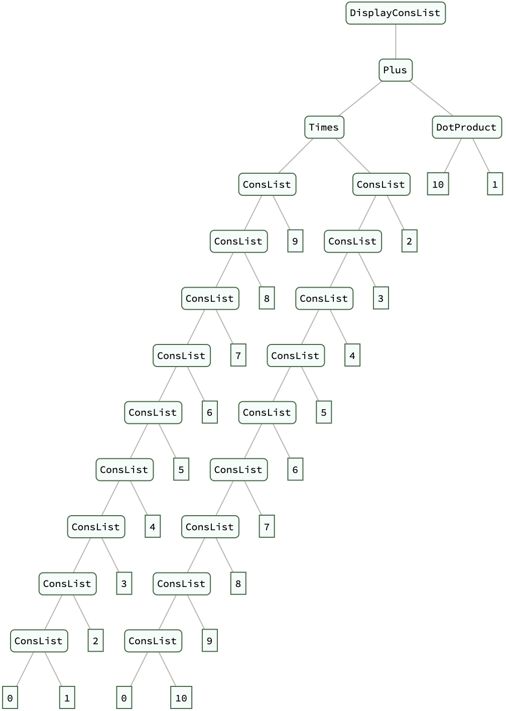
list1 = Fold[ConsList, 0, Range[10]];
list2 = Fold[ConsList, 0, Reverse[Range[10]]];
dotProductResult = DotProduct[list1, list2];
DisplayConsList[dotProductResult] // ExpressionTree

What is the suite of functions for expanding, mapping, partitioning, and selecting elements within these self-referential structures that we use to manipulate them? We can expand, map, partition, and select elements within these self-referential structures; ExpandConsList and DisplayConsList are introduced to visualize the growth of these structures up to a certain point. You've got to..appreciate the framework's ability to handle the Fibonacci sequence..we could recognize the potential for these structures to simplify complex data manipulation tasks significantly. What is the algorithmic complexity and efficiency of the operations defined within the framework? While linked lists typically offer certain computational advantages (like constant time for appending elements)..it's crucial to ensure that these benefits are preserved in the newly introduced data structures.
BlockchainNode[value_, next_] := <|"Value" -> value, "Next" -> next|>
CreateBlockchain[data_List] :=
 Fold[BlockchainNode, Last[data], Reverse[Most[data]]]
CoefficientOfRestitution[m1_, v1_, m2_, v2_] :=
 Abs[(v2 - v1)/(PreCollisionVelocity[m1, m2, v1, v2] -
     PreCollisionVelocity[m1, m2, v2, v1])]
PreCollisionVelocity[m1_, m2_, v1_, v2_] := (m1 v1 + m2 v2)/(m1 + m2)
SquareNumbers[n_] := Array[#^2 &, n]
TriangularNumbers[n_] := Array[(#*(# + 1))/2 &, n]
FibonacciUnprotected[n_] := Module[{fib}, fib[1] = 1; fib[2] = 1;
  fib[x_] := fib[x] = fib[x - 1] + fib[x - 2];
  Array[fib, n]]
MapConsTree[func_, tree_ConsTree] := TreeMap[func, tree]
ConsList /:
 DotProduct[ConsList[ID1_, next1_], ConsList[ID2_, next2_]] :=
 ID1*ID2 + DotProduct[next1, next2]
DotProduct[ConsList[ID1_, _], ConsList[ID2_, _]] := ID1*ID2
blockchain = CreateBlockchain[Range[5]]
e = CoefficientOfRestitution[5, 2, 3, -1]
squares = SquareNumbers[10]
triangles = TriangularNumbers[10]
fibSeq = FibonacciUnprotected[10]

While the current implementation may not be the most efficient in terms of runtime complexity, it lays the groundwork for future optimizations. Ideally, linked lists should operate in linear time for traversal operations. And that is why our data structure operates in non-linear time, because otherwise we would have to cache computed values to avoid redundant calculations in the future. The fundamental questions that we have about data structures, efficiency, and programming...it's a "common misrepresentation" of the Sieve of Eratosthenes algorithm that, in the context of lazy functional programming..it's the classic algorithm for finding all prime numbers up to a certain limit, and it has often been used to demonstrate how elegant this functionally is, what we're doing with this lazy evaluation in functional programming languages such as Haskell.
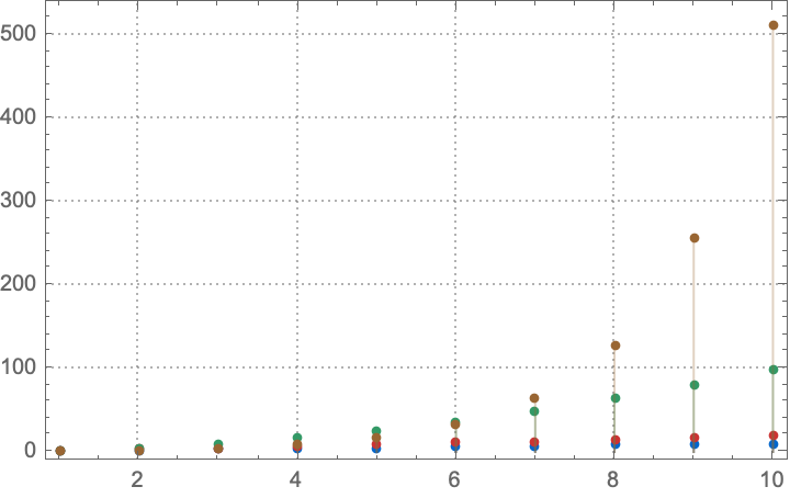
With[{infiniteOdds = ConsListRange[1, 2],
  infinitePowersOfTwo = InfiniteSteps[Times, 1, 2],
  firstTenIntegers = Take[ConsListRange[], 10],
  mappedIntegers = Map[#^2 &, ConsListRange[]],
  colors = {
    RGBColor[0, 0.4, 0.8],
    RGBColor[0.8, 0.2, 0.2],
    RGBColor[0.2, 0.6, 0.4],
    RGBColor[0.6, 0.4, 0.2]}},
 Show[
  MapThread[
   ListPlot[
     Take[#1, 10],
     Filling -> Axis,
     PlotTheme -> "Detailed",
     PlotStyle -> #2] &,
   {{firstTenIntegers,
     infiniteOdds,
     mappedIntegers,
     infinitePowersOfTwo},
    colors}
   ], PlotRange -> All]]
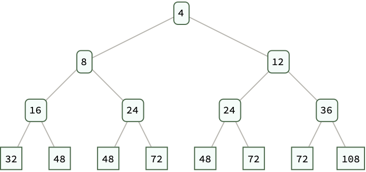
tree = NestConsTree[Function[x, {2*x, 3*x}], 4]
displayedTree = RootTree[tree, 3]

The "simplistic and elegant appearance of the code" belies its inefficiency, in the sense that the Sieve of Eratosthenes is, in fact, not the sieve but a form of the trial division algorithm, which "should only", show that for the traditional Sieve of Eratosthenes, for a given prime number p, multiples of p are marked as non-prime starting from p^2, since smaller multiples would have been marked by smaller primes. In contrast, the Haskell code often presented as the sieve is unfaithful to this method. The reason is that the Haskell code, what it actually does is it generates candidates for primes and filters out non-primes by checking divisibility against all previously found primes and that, is computationally more expensive. And that is how we got here @Athina Kyriazi, the kernel of Mathematica exists so that we can open another window - sure Mathematica isn't perfect, whatever that means but, it's..something else. Do you want O'Neill to provide a detailed analysis of Mathematica? It's full of convenience features.
With[{Sieve = Function[n,
    Module[{primes = Range[2, n], i = 1, p},
     While[(p = primes[[i]]) <= Sqrt[n],
      primes = DeleteCases[primes, x_ /; x != p && Mod[x, p] == 0];
      i++];
     primes]
    ],
  fibonacciNumbers =
   Take[InputSequence[#1 + #2 &, {# - 1, # - 2} &, {1, 1}], 13]
  },
 Module[{primesUpTo200 = Sieve[200],
   primeFibonacciNumbers = Select[fibonacciNumbers, PrimeQ],
   min,
   max},
  min = Min[primesUpTo200];
  max = Max[primesUpTo200];
  ListPlot[primesUpTo200,
   PlotStyle -> Directive[PointSize[Medium], Black],
   PlotRange -> {{1, Length[primesUpTo200]}, {min, max + 70}},
   Frame -> True,
   FrameLabel -> {"Index", "Value"},
   FrameStyle -> GrayLevel[0.1],
   GridLines -> {None, primeFibonacciNumbers},
   GridLinesStyle ->
    Directive[Thin, Dashed, RGBColor[0.4, 0.6, 0.8]],
   PlotLegends -> Placed[{"Prime Numbers Up to 200"}, {1, 0.8}],
   ImageSize -> 600,
   PlotTheme -> "Detailed"]
  ]]
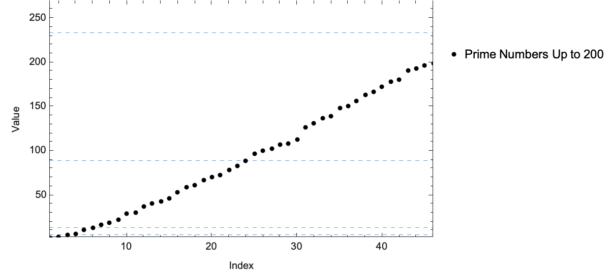
Will there be some different form of summarization of the world that's different than we imagine it? There's iconography there's user interfaces..those over the last few decades have come to be another level of a kind of communication to humans; there's certain kinds of things that the user interface can communicate and it's a little different, and a picture is worth a thousand words..although they don't have the same kind of compositionality that language seems to have, apparently. And we start to poke at communication and it gives a kind of sense of where one might see kinds of ways of packaging ideas, thoughts, that is very different from what we humans come up with, possibly, will the thing come up with be something that humans can learn?
ConsList /: KeyValue[ConsList[key_, value_], keys_List] :=
 If[MemberQ[keys, key], {key -> value}, KeyValue[value, keys]]
ledger =
  Fold[ConsList, {}, {{"Alice", 50}, {"Bob", -50}, {"Alice",
     25}, {"Bob", -25}}];
DisplayConsList[ledger] // ExpressionTree
KeyValue[ledger, {"Alice", "Bob"}]
bounce[height_, coeff_, limit_] :=
 NestWhileList[#*coeff &, height, # > limit &]
bounceHeights = bounce[10, 0.7, 0.1];
ListPlot[bounceHeights, Joined -> True, PlotMarkers -> Automatic,
 AxesLabel -> {"Bounce", "Height"}]
ConsTree /: Achieve[ConsTree[degree_, reqs_], degreeWanted_] :=
 If[degree === degreeWanted, degree,
  Achieve[#, degreeWanted] & /@ reqs]
educationTree =
 ConsTree["PhD", {ConsTree["Masters", {ConsTree["Bachelor", {}]}]}]
Achieve[educationTree, "Masters"]
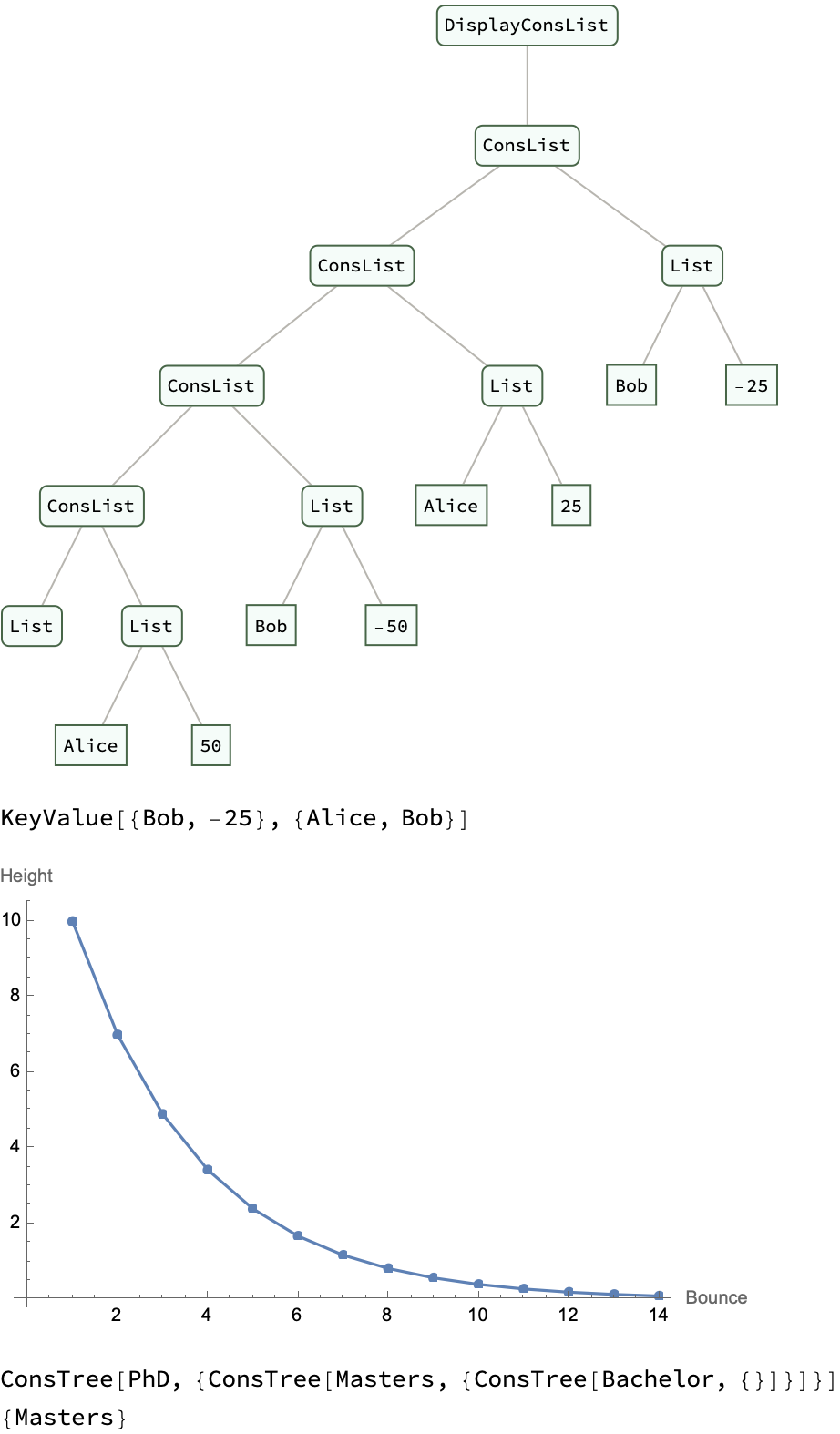
Because it's really about O'Neill, you know how the unfaithful sieve and the genuine sieve..the unfaithful sieve has a time complexity of O(n^2 / (log n)^2), which is significantly worse than the genuine sieve's O(n log log n)..and it's really the author who provides an implementation of the genuine sieve in Haskell that uses appropriate data structures to efficiently cross off multiples of primes, akin to the original sieve's process. And that should start to almost begin to explain how we reset the value of a variable. We do it without restarting the Evaluation kernel.
n = ConsListRange[];
binaryTree = NestConsTree[Function[x, {2*x, 3*x}], 4] ;
mapAt = MapAt[Function[x, 100], n, 2];
mapped = Map[Function[x, x^2], Take[n, 10]];
treeMapped = TreeMap[Function[x, 2*x], binaryTree, {0, 1, 2, 3}];
selected = Select[Take[n, 20], Function[x, EvenQ[x]]];
partitioned = Partition[Take[n, 10], 3];
oddNumbers = ConsListRange[1, 2];
evenNumbers = ConsListRange[2, 2];
riffled = Riffle[Take[oddNumbers, 5], Take[evenNumbers, 5]];
foldedList = FoldList[Plus, Take[n, 10]];
firstPosition = FirstPosition[n, 5];
Grid[{
  {"MapAt", "Mapped", "TreeMap"},
  {mapAt, mapped, treeMapped},
  {"Select Even", "Partition", "Odd Numbers"},
  {selected, partitioned, oddNumbers},
  {"Even Numbers", "Riffle", "FoldList"},
  {evenNumbers, riffled, foldedList},
  {"First Position", "Tree"},
  {firstPosition, tree}
  }, Frame -> All]
expressionTree =
 DisplayConsList[binTree, {0, 1, 2, 3}] // ExpressionTree

Performance in practice shows that while the unfaithful sieve is more straightforward to implement using lists in Haskell, it performs poorly in comparison to the genuine sieve, especially as the numbers involved grow larger. And that's why it's so important to choose the right data structure for the task at hand, which can make a significant difference in performance. This 2D infinity is so dreamy I don't know how else to put it, I can't believe this is happening, actually. It's O'Neill who goes further to introduce an improved implementation of the genuine sieve using a priority queue (or heap) instead of a list or tree to store the next composite numbers, which "increases" efficiency. She also discusses the use of a "wheel" optimization to skip multiples of small primes like 2, 3, 5, and 7, thereby reducing the number of candidates to be tested for primarily and improving performance even more.
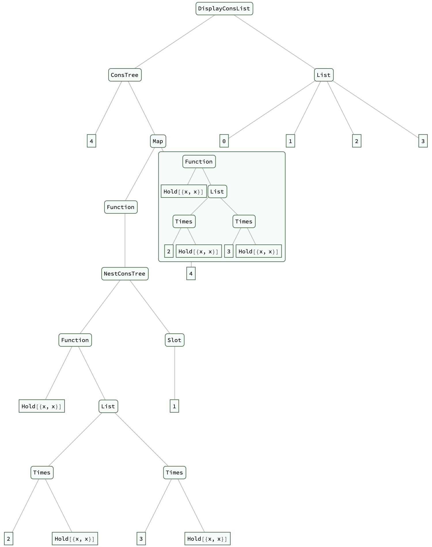
Furthermore, in Mathematica there are all kinds of keyboard shortcuts to complete the kernel. The paper itself, which clarifies what happens when we quit the kernel, clarifies a long-standing confusion in the functional programming community, demonstrating that with careful consideration of algorithmic design and data structures, one can implement the Sieve of Eratosthenes efficiently in a lazy functional style. The work encourages functional programmers to explore beyond lists and to utilize more complex data structures when they are more suitable for the problem at hand.
nExternal = 10;
primeNumbers = Map[Log[#] &,
   Take[primes, 15]];
fibonacciNumbers = Map[Log[#] &,
   Take[fib, 30]];
nestedSequences = Map[Log[#] &,
   Take[Map[Take[#, nInternal] &,
     Map[NestConsList[f, #] &, ConsListRange[1, 1]]],
    nExternal],
   {2}];
squaredSequences = Map[Log[#] &,
   Take[Map[Take[#, nInternal] &,
     Map[NestConsList[#^2 &, #] &,
      ConsListRange[1, 1]]],
    nExternal],
   {2}];
Show[MapThread[
  ListPlot[#1,
    PlotMarkers -> Automatic,
    Frame -> True,
    Joined -> True,
    GridLines -> Automatic,
    GridLinesStyle -> Directive[Gray, Dashed],
    ImageSize -> Large,
    PlotStyle -> #2,
    PlotLegends -> {#3},
    PlotRange -> {Automatic,
      {Min[squaredSequences],
       Max[squaredSequences]}}
    ] &,
  {{primeNumbers,
    fibonacciNumbers,
    nestedSequences,
    squaredSequences},
   {RGBColor[0.6, 0.3, 0.5],
    RGBColor[0.2, 0.55, 0.4],
    RGBColor[0.9, 0.5, 0.5],
    RGBColor[0.5, 0.7, 0.9]},
   {"Prime Numbers",
    "Fibonacci Numbers",
    "Nested Sequences",
    "Squared Sequences"}}]]
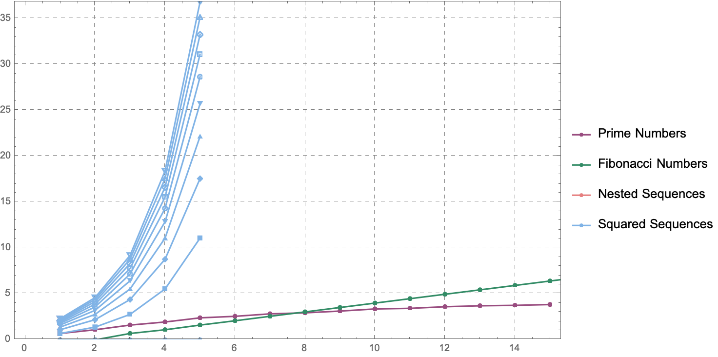
@Athina Kyriazi For the better, the potential to transform the world these prime numbers have at a scale that, can I imagine it? No. It's even not about how foliation has to not be with respect to time, or whether it can be some arbitrary other spatial parameter. This framework is for the linked list data structure: the "practice" of critically evaluating the performance and faithfulness of algorithms, especially when teaching or employing them as exemplars of programming paradigms, demonstrates the relevance of algorithmic design and the thoughtful use of data structures in the realm of functional programming where lists and one-liners are often (mis)presented as the de facto tools for all tasks.
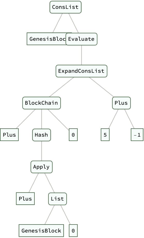
BlockChain[head_, data_, step_] :=
 ConsList[data, BlockChain[head, Hash[head @@ {data, step}], step]]
simpleChain = BlockChain[Plus, "GenesisBlock", 0];
Print[ExpandConsList[simpleChain, 5] // ExpressionTree]
CollisionModel[m1_, m2_, v1i_, v2i_, e_] :=
 Module[{v1f, v2f},
  v1f = (e*m2*(v2i - v1i) + m1*v1i + m2*v2i)/(m1 + m2);
  v2f = (e*m1*(v1i - v2i) + m1*v1i + m2*v2i)/(m1 + m2);
  {v1f, v2f}]
EducationTree[course_] :=
 ConsTree[course, EducationTree /@ PrerequisiteCourses[course]]
PrerequisiteCourses[course_] :=
 Switch[course, "Calculus", {"Algebra", "Geometry"},
  "Algorithms", {"Data Structures", "Discrete Math"},
  "Machine Learning", {"Statistics", "Algorithms"}, _, {}]
mlPrerequisites = EducationTree["Machine Learning"];
DisplayConsList[mlPrerequisites, {0, 1, 2}] // ExpressionTree

And that's why it's so important to choose the right data structures and architecture to look beyond surface-level elegance and simplicity. The concept of a "wheel" to skip over numbers that are multiples of the first few primes..by using this technique, the implementation reduces the number of candidates and computations required, thereby optimizing the sieve process..in order to rectify the misinformation I uh, ought to provide an actual implementation of the Sieve of Eratosthenes by Haskell that utilizes more complex data structures, what with the original sieve and its method of eliminating non prime numbers and doing so with improved efficiency.
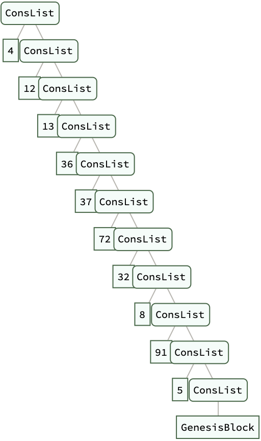
AppendBlock[ledger_ConsList, data_] := ConsList[data, ledger];
Blockchain :=
  Nest[AppendBlock[#, RandomInteger[100]] &, ConsList[GenesisBlock],
   10];
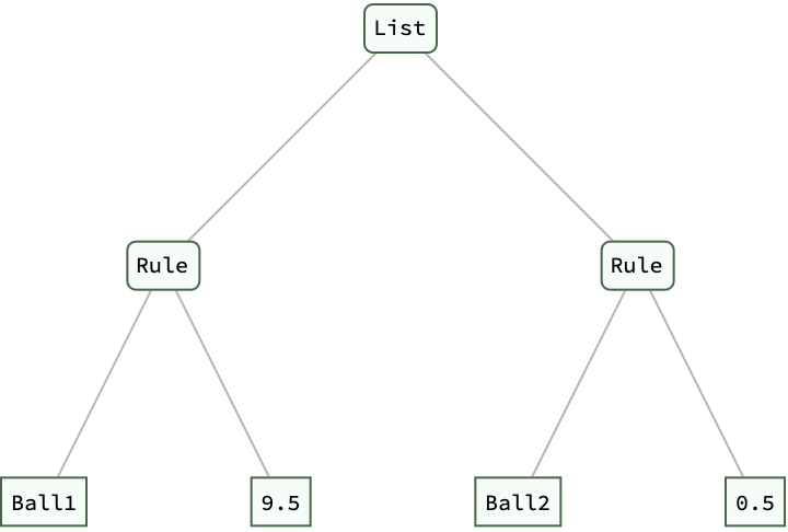
Collision[k1_, m1_, u1_, k2_, m2_, u2_, e_] :=
  Module[{v1, v2}, v1 = (e*m2*(u2 - u1) + m1*u1 + m2*u2)/(m1 + m2);
   v2 = (e*m1*(u1 - u2) + m1*u1 + m2*u2)/(m1 + m2);
   {k1 -> v1, k2 -> v2}];
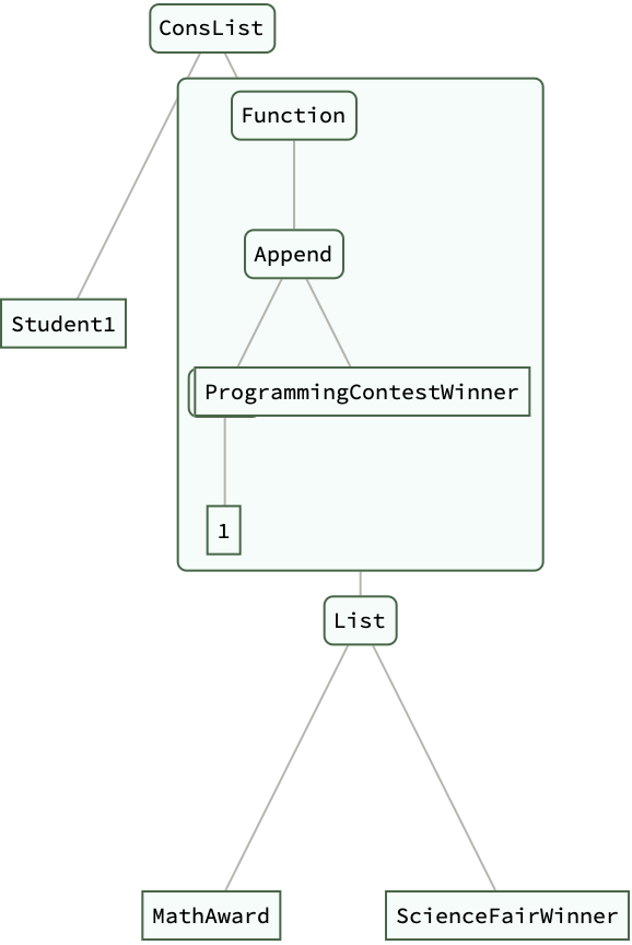
RecordAchievements[student_ConsList, achievement_] :=
  MapAt[Append[#, achievement] &, student, -1];
Framework[func_, initialData_, steps_] :=
  Nest[func, initialData, steps];
ledger = Blockchain;
studentAchievements =
  ConsList["Student1", {"MathAward", "ScienceFairWinner"}];
updatedStudentAchievements =
  RecordAchievements[studentAchievements,
   "ProgrammingContestWinner"];
collisions = Collision["Ball1", 1, 0, "Ball2", 1, 10, 0.9];
ledger // ExpressionTree
updatedStudentAchievements // ExpressionTree
collisions // ExpressionTree
What is the "true" time complexity of both the genuine and unfaithful sieve? The genuine Sieve of Eratosthenes exhibits a linearithmic time "complexity" of O(n log log n), while the unfaithful sieve exhibits a quadratic time complexity relative to the logarithm of the number, O(n^2 / (log n)^2). The practical performance results we should do reproduce (in both theory and practice) the superiority of the genuine sieve. The Haskell code is inefficient, and that's why it's inefficient, because it's inefficient because it performs unnecessary divisibility checks. These divisibility checks are unnecessary, because it tests every number against all previously identified primes in all possibilities rather than strategically eliminating multiples from a list, which results in significantly slower execution on a scale of time complexity, especially only and unless we use larger lists of numbers.
SetAttributes[ConsList, HoldAllComplete];
SetAttributes[ConsTree, HoldAllComplete];
BlockChain[value_, nextBlock_] := ConsList[value, nextBlock];
CreateBlock[previousBlock_, transaction_] :=
  BlockChain[Hash[{previousBlock, transaction}], previousBlock];
GenerateBlockchain[n_Integer] :=
  Nest[CreateBlock[#, RandomChoice[{"Tx1", "Tx2", "Tx3"}]] &,
   BlockChain[Hash["Genesis"], None], n];
blockchain = GenerateBlockchain[10];
VerifyBlockchain[BlockChain[_, None]] := True;
VerifyBlockchain[BlockChain[hash_, prevBlock_]] :=
  hash === Hash[{prevBlock, First@prevBlock}] &&
   VerifyBlockchain[prevBlock];
verified = VerifyBlockchain[blockchain]
CoefficientOfRestitution[m1_, v1_, m2_, v2_, e_] :=
  Solve[m1 v1 + m2 v2 == m1 v1' + m2 v2' &&
    e == (v2' - v1')/(v1 - v2), {v1', v2'}];
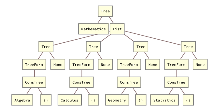
EducationTree[subject_, topics_] := ConsTree[subject, topics];
mathTopics = {"Algebra", "Calculus", "Geometry", "Statistics"};
mathTree =
  EducationTree["Mathematics", EducationTree[#, {}] & /@ mathTopics];
DisplayEducationTree[ConsTree[subject_, topics_]] :=
  TreeForm[Tree[subject, TreeForm /@ topics]];
mathTreeDisplayed = DisplayEducationTree[mathTree]

And I guess that's the computational wheel that we'll find buried in the paper, the numbers that are multiples of the first few primes we can skip over with the wheel. By using this technique, the implementation reduces the number of candidates and computations required, thereby optimizing the sieve process. A widely circulated Haskell "one-liner" generates prime numbers but it is not the genuine Sieve of Eratosthenes. It is in fact an unfaithful representation that corresponds more closely to trial division. The beauty and simplicity is dismantled, in the sense that the code is efficient and faithful just not to the original algorithm devised by Eratosthenes. That's how we got all those quantum tutorials it really made me smile.
BlockChain[data_] :=
 Nest[ConsList[Hash[#], #] &, ConsList[Hash[data], data],
  Length[data]]
data = {"Block 1", "Block 2", "Block 3"};
chain = BlockChain[data] // ExpressionTree

The commonly used Haskell code may very well be the amazing gemstone. It performs divisibility checks. It tests every number against primes previously identified. There's some kind of scaling, the actual neurons in the physical brain, the number of neurons in the brain and the number of distinct words that can be dealed with, how many words can an ant deal with it has 50,000 neurons, the ant can perhaps communicate. The question becomes, if we start to have neural nets that have 10 to the trillion neurons in them, if we take what we see from the world, this collection of different images, they will correspond to this concept. How many attractors, or is it the case that if our brain has a certain number of neurons and we want to pack more and more concepts, because the sort of attractor, the pattern of brain activity that we recognize as the concept of cat, the pattern of brain activity that we recognize as the concept of dog..they'll start to be overlapped and you'll start to not be able not to distinguish between those things.
BlockConsList[data_, nextBlock_ : None] := ConsList[data, nextBlock]
AddBlock[blockchain_, data_, hashFunction_] :=
 Module[{newBlock, lastBlockHash},
  lastBlockHash = hashFunction[Last[blockchain]];
  newBlock = BlockConsList[{data, lastBlockHash}];
  Append[blockchain, newBlock]]
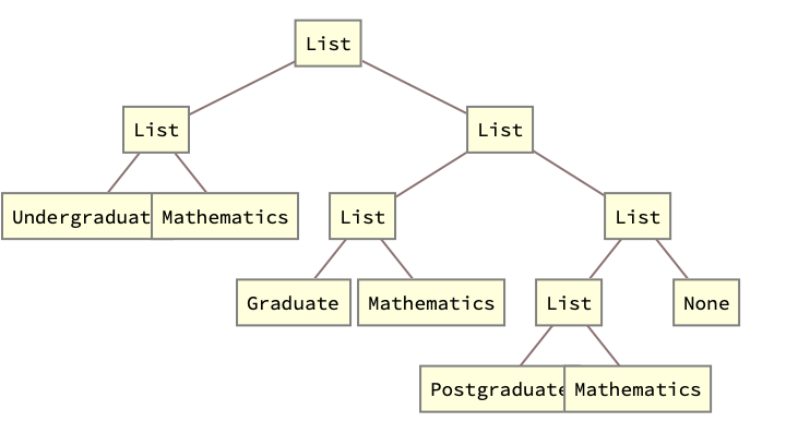
EducationalTree[level_, subject_, next_ : None] :=
 ConsTree[{level, subject}, next]
BuildCurriculum[subject_, levels_] :=
 Fold[EducationalTree[#2, subject, #1] &, None, Reverse@levels]
CalculateCollisionOutcome[mass1_, velocity1_, mass2_, velocity2_,
  restitutionCoefficient_] := {finalVelocity1, finalVelocity2}
DisplayStructure[structure_] :=
 TreeForm[structure /. ConsList | ConsTree -> List]
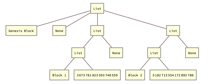
blockchain = BlockConsList["Genesis Block"];
blockchain = AddBlock[blockchain, "Block 1", Hash];
blockchain = AddBlock[blockchain, "Block 2", Hash];
curriculumTree =
  BuildCurriculum[
   "Mathematics", {"Undergraduate", "Graduate", "Postgraduate"}];
collisionOutcome = CalculateCollisionOutcome[2, 3, 5, -1, 0.8];
DisplayStructure[blockchain]
DisplayStructure[curriculumTree]
collisionOutcome

I think that your framework for handling self referential data structures just shows how we perform operations on them, and then we can reflect on the operations that we are performing which are meant to illustrate how we create and manipulate infinite data structures in a functional programming style. That's how the arguments for the ConsList and the ConsTree symbols have been held unevaluated..what with the arguments that matter for creating self referential structures..we can prevent infinite recursion by resting. I think that we have a clear choice..we can define an infinite list, or stream that starts with init and then successively applies head to generate the next element using the previous element and step. Then, we can generate a self referential structure, using a seed list and a function func that determines how each new element is computed from previous ones. The recursive structure is built using Fold and ReplaceAll, which is symbolized by the /.. And then we can create an infinite list.
SetAttributes[ConsList, HoldRest];
SetAttributes[ConsTree, HoldRest];
InfiniteSteps[head_, init_, step_] :=
  ConsList[init, InfiniteSteps[head, head[init, step], step]];
GenerateSequence[func_, seed_List] :=
  Fold[ConsList[#2, #] &, ConsList[Last[seed], Null],
    Reverse[Most[seed]]] /.
   Null -> (ConsList[func @@ Take[%, Length[seed]], #0] &);
fibonacciSeq = GenerateSequence[Plus, {0, 1}];
MapConsList[f_, ConsList[head_, tail_]] :=
  ConsList[f[head], MapConsList[f, tail]];
NestConsTree[f_, init_, depth_] :=
  ConsTree[init,
   If[depth > 1, NestConsTree[f, #, depth - 1] & /@ f[init], {}]];
binaryTree = NestConsTree[{2 # &, 3 # &}, 1, 3];
MapConsTreeLevel[f_, tree_ConsTree, level_Integer] :=
  Map[f, TreeLevel[tree, level], {level}];
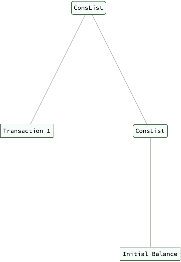
AppendTransaction[ledger_ConsList, transaction_] :=
  ConsList[transaction, ledger];
Bounce[height_, restitution_] :=
  NestWhileList[# restitution &, height, # > 0.01 &];
AddEducation[person_Association, degree_] :=
  Append[person, "Education" -> degree];
ledger = ConsList["Initial Balance"];
ledger = AppendTransaction[ledger, "Transaction 1"] // ExpressionTree
bounces = Bounce[10, 0.9];
person = <|"Name" -> "Alice"|>;
person = AddEducation[person, "PhD in Physics"]

We can represent the Fibonacci sequence using the GenerateSequence function. If we didn't need vectorization then we could just do iterative programming. But in Mathematica, we can actually do the "closed form" function application of a given function f to each element of a ConsList, effectively mapping f over the list. The NestConsTree function generates a self referential tree structure with a given depth, where f is a function (or list of functions, since we're doing vectorized) generation of the children of each node in the tree.
SimpleHash[data_, prevHash_] := Mod[Hash[data] + prevHash, 10^10]
CreateGenesisBlock[data_] :=
 BlockChain[SimpleHash[data, 1], data, "Genesis", Null]
AddBlock[chain_BlockChain, data_] :=
 BlockChain[SimpleHash[data, chain["Hash"]], data, chain,
  chain["Prev"]]
BlockChain /: BlockChain[hash_, _, _, _]["Hash"] := hash
BlockChain /: BlockChain[_, _, prev_, _]["Prev"] := prev
genesisBlock = CreateGenesisBlock["Linked List Emulation"]
block2 = AddBlock[genesisBlock, "Lazy Infinite Evaluation"]
block3 =
 AddBlock[block2,
  "Make a framework for self referential data structures"]
block4 =
 AddBlock[block3,
  "Check the algorithmic complexity of various operations"]
ValidateChain[BlockChain[hash_, data_, "Genesis", _]] := True
ValidateChain[block_BlockChain] :=
 block["Hash"] ==
   SimpleHash[block["Prev"]["Data"], block["Prev"]["Hash"]] &&
  ValidateChain[block["Prev"]]
ValidateChain[block4]

There are a bunch of different words that a person might not know but which are useful for communicating medical concepts and that somehow leverage, go further with language than we could go with everyday words. And when we have a million word AI what it will sort of feel like to be able to deal with such a question we don't know, that was my thought with what sort of level we can understand a language - is there a form of language perhaps more efficient than language achievable by a thing that can keep more concepts of mind? It would be very hard to imagine what it would be like if one had language, and if one didn't have language.
BlockChain /:
 BlockChain[hash_, data_, prev_, restitution_][
  "Restitution"] := restitution
ComputeRestitution[block1_BlockChain, block2_BlockChain] :=
 RandomReal[{0, 1}]
block3 =
 AddBlock[block2,
  "Made a framework for self referential data structures",
  ComputeRestitution[block2, block3]]
block4 =
 AddBlock[block3,
  "Checked the algorithmic complexity of various operations",
  ComputeRestitution[block3, block4]]
block3["Restitution"]
block4["Restitution"]

Our computational language, Wolfram Language which didn't exist and does exist, we can begin to see how one can begin to clarify such things in its full form from the infinite data structures, the existence of computational language helps one think thoughts in a different way, compose thoughts in a different way, what it might feel like to deal with an AI that knows a million different words opens up possibilities for working with complex recursive structures and let's see, it emphasizes the balance between elegant code and practical runtime complexity, because what we're doing is we're using a lot of compression representing these infinite lists and trees in a manner that is computationally feasible. That's really a story of compression, a story of taking every pixel arrangement and just saying it's a camera!
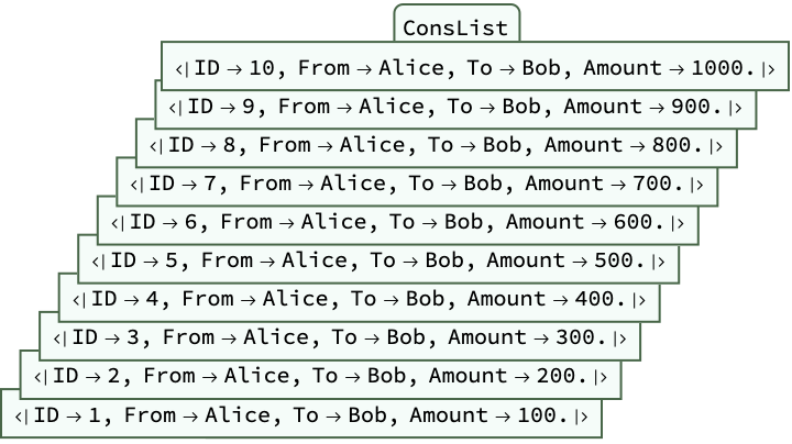
Transaction[id_Integer, from_String, to_String, amount_Real] := <|
   "ID" -> id, "From" -> from, "To" -> to, "Amount" -> amount|>;
CreateLedger[transactions_List] :=
  Fold[ConsList, "Genesis", transactions];
ledger =
 CreateLedger[
   Transaction[#, "Alice", "Bob", 100.0*#] & /@ Range[10]] //
  ExpressionTree
VerifyLedgerIntegrity[ConsList["Genesis", _]] := True
VerifyLedgerIntegrity[ConsList[Transaction[id_, _, _, _], next_]] :=
 id == 1 || (id - 1 == next[[1]]["ID"] && VerifyLedgerIntegrity[next])
Something where you've concentrated that into a thing that represents a sort of coherence that can be proved, like traversing or joining lists in constant or linear time, not quadratic or worse. The thing to understand about words, the precision of meaning, the whole point is the idea of compression. I could say it's a cameraloglalala and manipulate these structures with extended list-framework functions and new framework function definitions. Data structures with infinite recursive definitions can lead to errors due to exceeding recursion limits it's super scary when you see how self referential expressions can be operated upon meaningfully within computational frameworks. Things can happen every nanosecond. The fundamental hardware of our brains..are inspired by the functional programming concept of lazy evaluation, akin to constructs in Lisp.