That was sensationally unprecedented! When you're in vector calculus and optimization, you never know when you might need to showcase the power of the Lagrange Multipliers technique in multiple scenarios to show the critical points on these dimensional surfaces of the functions f and g, the auxiliary operations that can do so much with so little. It's "reminiscent" of referencing the CheckerBoard texture which is in "need" of a provider if it's supposed to exist, how do we need a provider.. that's why we enjoy this article [WSS22] Lecture notes for Vector Calculus it's an intuitive, insider's view for all mathematical solutions, with these visualizations.
f[x_, y_, z_] := x^2 + y^2 + z^2;
g[x_, y_, z_] := x + y + z - 3;
g1[x_, y_, z_] := x + y + z - 3;
g2[x_, y_, z_] := x^2 + y^2 - 1;
f2D[x_, y_] := x^2 + 2 y^2;
g2D[x_, y_] := x^2 + y^2;
d[x_, y_, z_] := x^2 + y^2 + z^2;
g3[x_, y_, z_] := x^2 - y^2 - z^2;
f3D[x_, y_, z_] := x^2 + y^2 + 2*z^2 - 3*x*y + 2*y*z - x*z;
g3D[x_, y_, z_] := x^2 + y^2 + z^2;
solution1 =
  N[Solve[Join[
     Thread[Grad[
        f[x, y, z], {x, y, z}] == \[Lambda] Grad[
         g[x, y, z], {x, y, z}]], {g[x, y, z] == 0}], {x, y,
     z, \[Lambda]}]];
solution2 =
  N[Solve[Join[
     Thread[Grad[
        f[x, y, z], {x, y,
         z}] == \[Lambda] Grad[g1[x, y, z], {x, y, z}] + \[Mu] Grad[
          g2[x, y, z], {x, y, z}]], {g1[x, y, z] == 0,
      g2[x, y, z] == 0}], {x, y, z, \[Lambda], \[Mu]}]];
solution3 =
  Solve[Join[
    Thread[Grad[
       f2D[x, y], {x, y}] == \[Lambda] Grad[g2D[x, y], {x, y}]], {g2D[
       x, y] == 1}], {x, y, \[Lambda]}];
solution4 =
  NMinimize[{8 x^2 + 4 y*z - 16 z + 600,
    4 x^2 + y^2 + 4 z^2 == 16}, {x, y, z}];
sol5 = Solve[{D[f2D[x, y], x] == \[Lambda] D[g2D[x, y], x],
    D[f2D[x, y], y] == \[Lambda] D[g2D[x, y], y], g2D[x, y] == 0}, {x,
     y, \[Lambda]}];
solution6 =
  Reduce[Join[
    Thread[Grad[
       d[x, y, z], {x, y, z}] == \[Lambda] Grad[
        g3[x, y, z], {x, y, z}]], {g3[x, y, z] == 1}], {x, y,
    z, \[Lambda]}];
contour =
  ContourPlot3D[{f[x, y, z], g[x, y, z]}, {x, -5, 5}, {y, -5,
    5}, {z, -5, 5}, Contours -> {1, 0},
   ContourStyle -> {Directive[Red, Opacity[0.5]],
     Directive[Blue, Opacity[0.5]]}];
points1 = {x, y, z} /. solution1;
points1Plot = Graphics3D[{PointSize[0.02], Point[points1]}];
points2 = Select[{x, y, z} /. solution2, FreeQ[#, _Complex] &];
points2Plot = Graphics3D[{PointSize[0.02], Point[points2]}];
points3 = {x, y} /. solution3;
points5 = {x, y} /. sol5;
isolatedPoints = Select[points6, AllTrue[#, NumericQ] &];
parametricCurves = Complement[points6, isolatedPoints];
points6Plot = Graphics3D[{PointSize[0.02], Point[isolatedPoints]}];
parametricPlots =
  If[MemberQ[parametricCurves, {_, y, _}],
   ParametricPlot3D[{0, y, -Sqrt[-1 - y^2]}, {y, -Sqrt[2], Sqrt[2]},
    PlotStyle -> {Green, Thick}], {}];
organizedPlots =
  Grid[{{Show[contour, points1Plot],
     Show[contour,
      points2Plot]}, {ContourPlot[{f2D[x, y] == 0,
       g2D[x, y] == 1}, {x, -5, 5}, {y, -5, 5},
      ContourStyle -> {Red, Blue},
      Epilog -> {PointSize[0.02], Point[points3]}],
     ContourPlot[{f2D[x, y] == 0, g2D[x, y] == 0}, {x, -5, 5}, {y, -5,
        5}, ContourStyle -> {Red, Blue},
      Epilog -> {PointSize[0.02], Point[points5]}]}, {Show[
      contourPlot6, points6Plot, parametricPlots]}}];
organizedPlots
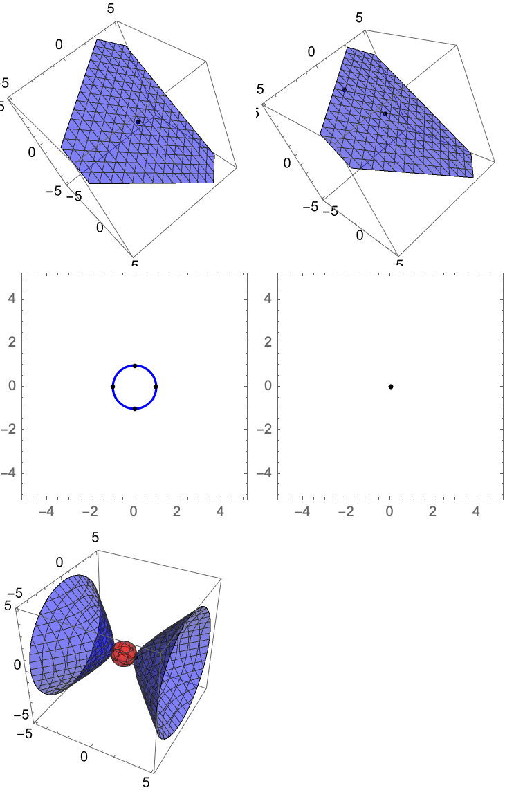
Solving those equations, getting the LaGrangian, doing the critical points..Your equations have some real value. This is an unparalleled field.. you've rejuvenated our trust in science with this post! Now when the probe lands on this scorched surface we can actually find the critical points, by doing the LaGrangian..The extreme values and the constraints.. and you know those grainy contour plots with these points and all. This has been some exploration!
ClearAll[x, y, z, \[Lambda], f3D, g3D];
f3D[x_, y_, z_] := x^2 + y^2 + 2*z^2 - 3*x*y + 2*y*z - x*z;
g3D[x_, y_, z_] := x^2 + y^2 + z^2;
solution3D =
Solve[Join[
Thread[Grad[
f3D[x, y, z], {x, y, z}] == \[Lambda] Grad[
g3D[x, y, z], {x, y, z}]], {g3D[x, y, z] == 1}], {x, y,
z, \[Lambda]}];
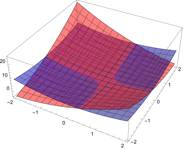
Show[Plot3D[f3D[x, y, z /. solution3D[[1]]], {x, -2, 2}, {y, -2, 2},
PlotStyle -> {Opacity[0.5], Red}],
Plot3D[g3D[x, y, z /. solution3D[[1]]], {x, -2, 2}, {y, -2, 2},
PlotStyle -> {Opacity[0.5], Blue}]]
ClearAll[x, y, \[Lambda], f, g];
f[x_, y_] := x^2 + 2 y^2;
g[x_, y_] := x^2 + y^2;
solution =
FindRoot[
Flatten[{Thread[
Grad[f[x, y], {x, y}] == \[Lambda] Grad[g[x, y], {x, y}]],
g[x, y] == 1}], {{x, RandomReal[{-2, 2}]}, {y,
RandomReal[{-2, 2}]}, {\[Lambda], RandomReal[{-2, 2}]}}];
h[x_, y_] := x^3 - 3 x*y^2;
gradh = Grad[h[x, y], {x, y}];
The thing is nothing and you've got these lecture notebooks in classrooms, our little munchkins incorporate real live interactive content. It's not your fault that in all these live optimization problems there's a constraint, that's the primary focus on the Lagrange multipliers method. I always wondered how these variables can take on different values, and apparently they really are variables; the mathematical example where the function f(x,y) = 2x + 2^2 y is subject to the constraint g(x,y) = 2x + 2y. Never mind..now this solution is an example..compute the gradients of f & g and you get the scalar multiple of the gradient of g via Lagrange multipliers after and ever since you equate the gradient of f to the gradient of g via the scalar multiple, there you will find the maximum value. Whenever you find these example solutions, centuries pass.
f[x_, y_] := Sin[x*y];
g[x_, y_] := x^2 + y^2;
gradf = Grad[f[x, y], {x, y}];
gradg = Grad[g[x, y], {x, y}];
lagrange = Thread[Equal[gradf, \[Lambda] gradg]];
constraint = g[x, y] == 1;
solution = Solve[Join[lagrange, {constraint}], {x, y, \[Lambda]}];
realSolutions = Select[solution, FreeQ[#, _Complex] &];
pts = {x, y} /. realSolutions;
ContourPlot[{f[x, y], g[x, y] - 1}, {x, -2, 2}, {y, -2, 2},
 Contours -> {Automatic, {1}}, ContourShading -> {Automatic, None},
 ContourStyle -> {Automatic, {Thick, Blue}},
 Epilog -> {Red, PointSize[0.015], Point[pts], Arrowheads[0.025],
   Arrow[{{#1, #2}, {#1, #2} + 0.5 Normalize[gradf] /. {x -> #1,
         y -> #2}}] & @@@ pts, Green,
   Arrow[{{#1, #2}, {#1, #2} + 0.5 Normalize[gradg] /. {x -> #1,
         y -> #2}}] & @@@ pts}, PlotLegends -> {"f(x,y)", "g(x,y)=1"}]
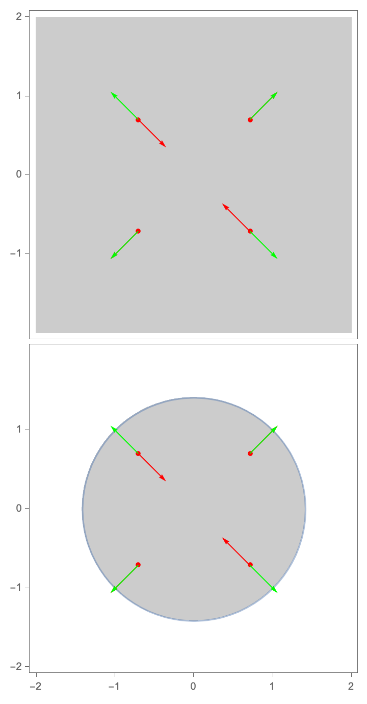
The assumption that we can equate the gradient of f to the gradient of g and find the critical points by the resulting system of equations solution, don't get too attached. Supposedly this system of equations yields different solutions depending on the multiplier, and even when you have the same multiplier, the solution changes depending on the constraint, at the time. So with the method of Lagrange multipliers where we plot the function over a domain, and the contour plots, the meaning is that this is nothing more than a systematic procedure in that we visualize the functions and, with all this educational material on Lagrange multipliers that we practice, we can focus on the method of Lagrange multipliers.
f[x_, y_] := Sin[x*y];
g[x_, y_] := x^2 + y^2;
solutions = {{1/Sqrt[2], -1/Sqrt[2]}, {-1/Sqrt[2],
    1/Sqrt[2]}, {-1/Sqrt[2], -1/Sqrt[2]}, {1/Sqrt[2], 1/Sqrt[2]}};
Show[Plot3D[f[x, y], {x, -1.5, 1.5}, {y, -1.5, 1.5},
  MeshFunctions -> {#3 &}, Mesh -> {{0}}, MeshStyle -> {{Thick, Red}},
   PlotRange -> All, BoxRatios -> {1, 1, 1},
  AxesLabel -> {"x", "y", "f(x,y)"}],
 ParametricPlot3D[{Cos[\[Theta]], Sin[\[Theta]],
   f[Cos[\[Theta]], Sin[\[Theta]]]}, {\[Theta], 0, 2 \[Pi]},
  PlotStyle -> {Blue, Thick}],
 Graphics3D[{Green, PointSize[Large],
   Point[{{#[[1]], #[[2]], f[#[[1]], #[[2]]]}}] & /@ solutions}]]
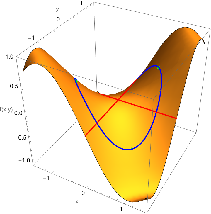
Let's suppose we want to find the max/min of a function given a constraint, it will just be so great. Compute the gradient of the function and its constraint, set them equal by a multiplier, and then you're ready to solve for critical points. Now, we want to find extreme values, so we confiscate f(x,y) = 2x + 2^2 y the function subject to g(x,y) = 2x + 2y the constraint. Then again, we could probably do this for any type of function because this is all fake, now, f(x,y) has an absolute max of 2 at (0,+/- 1) and an absolute min of 1 at (+/- 1, 0). Right @Passant Abbassi ? After all this system of equations solution doesn't have an expiration date. There will always be some minimum distance to find.
d[x_, y_, z_] := Sin[x*y*z];
g[x_, y_, z_] := x^2 + y^2 + z^2;
gradd = Grad[d[x, y, z], {x, y, z}];
gradg = Grad[g[x, y, z], {x, y, z}];
lagrange = Thread[Equal[gradd, \[Lambda] gradg]];
system = Flatten[{lagrange, g[x, y, z] == 1}];
solutions = Solve[system, {x, y, z, \[Lambda]}, Reals];
Graphics3D[{{Opacity[0.5], Sphere[]}, {Red, PointSize[0.02],
   Point[{x, y, z} /. solutions]}}, Axes -> True, Boxed -> True,
 PlotRange -> {{-1.5, 1.5}, {-1.5, 1.5}, {-1.5, 1.5}},
 Lighting -> "Neutral"]
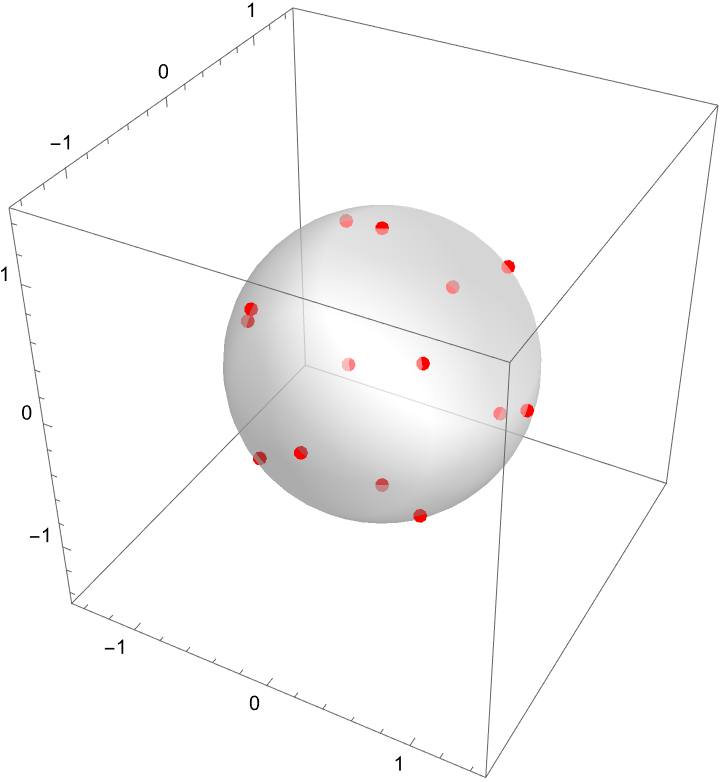
Last but not least, now's the time to create some context. Okay I understand that a space probe shaped like an ellipsoid enters Earth's atmosphere and starts heating. After 1 hour, its temperature at a point on its surface is represented by Θ. Coincidence? No, the hottest point on the probe's surface is "also" determined by the function to maximize...Θ(x,y,z) = 8^2 x + 4yz - 16z + 600 subject to the constraint g(x,y,z) = 4^2 x + 2y + 4^2 z = 16, but not for long; the solution involves applying the method of Lagrange multipliers, to quickly find the values of x, y, z and λ.
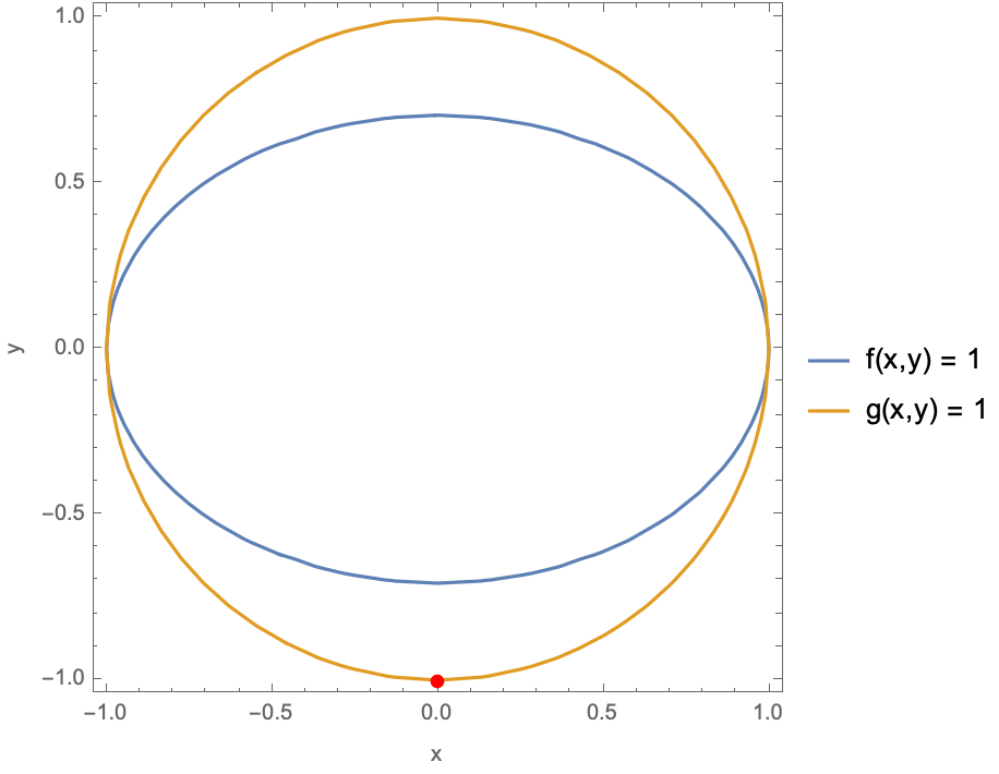
ClearAll[x, y, z, \[Lambda]];
f[x_, y_] := x^2 + 2 y^2;
g2D[x_, y_] := x^2 + y^2;
solution2D =
Solve[{Grad[f[x, y], {x, y}] == \[Lambda] Grad[g2D[x, y], {x, y}],
g2D[x, y] == 1}, {x, y, \[Lambda]}];
ContourPlot[{f[x, y] == 1, g2D[x, y] == 1}, {x, -2, 2}, {y, -2, 2},
Epilog -> {Red, PointSize[0.02],
Point[{x, y} /. Flatten[solution2D]]},
PlotLegends -> {"f(x,y) = 1", "g(x,y) = 1"}, PlotRange -> All,
FrameLabel -> {"x", "y"}]
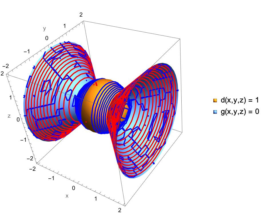
d[x_, y_, z_] := x^2 + y^2 + z^2;
g3D[x_, y_, z_] := x^2 - y^2 - z^2;
solution3D =
Solve[{Grad[
d[x, y, z], {x, y, z}] == \[Lambda] Grad[
g3D[x, y, z], {x, y, z}], d[x, y, z] == 1}, {x, y,
z, \[Lambda]}];
parametricCurve =
ParametricPlot3D[{x, y, z} /.
Select[solution3D, ! FreeQ[#, y] &], {y, -1, 1},
PlotStyle -> {Green, Thick}];
Show[ContourPlot3D[{d[x, y, z] == 1, g3D[x, y, z] == 0}, {x, -2,
2}, {y, -2, 2}, {z, -2, 2},
MeshFunctions -> {Function[{x, y, z, f}, d[x, y, z] - 1],
Function[{x, y, z, f}, g3D[x, y, z]]},
MeshStyle -> {{Thick, Red}, {Thick, Blue}}, BoundaryStyle -> None,
PlotLegends -> {"d(x,y,z) = 1", "g(x,y,z) = 0"},
AxesLabel -> {"x", "y", "z"}], parametricCurve]
The Wolfram Language, we can perfectly understand it as it crystallizes, each step in the problem-solving process, the contour plots and visualization of functions. Actually, the real question I should be asking is, do I like calculating the critical points using the method of Lagrange multipliers? The explanation, nothing makes sense anymore! First define the function, compute the gradient, apply the Lagrange multipliers, and then the critical points will crystallize not only and not unless we provide more visualizations related to critical point computations, to admire the depth of science and exploration in [WSS22] Lecture notes for Vector Calculus.
ClearAll[x, y, z];
contourPlotf1 = ContourPlot[x^2 + y^2 + 1, {x, -2, 2}, {y, -2, 2}];
gradf2 = Grad[x^2 + 2 y^2, {x, y}];
combined3Df2 =
  Show[Plot3D[x^2 + 2 y^2, {x, -2, 2}, {y, -2, 2}, Mesh -> None],
   Graphics3D[
    Table[Arrow[{{x, y, x^2 + 2 y^2}, {x, y, x^2 + 2 y^2} +
        Append[0.1 Normalize[gradf2], 0.1 Norm[gradf2]]}], {x, -2, 2,
      0.2}, {y, -2, 2, 0.2}]]];
data = NestList[{Surd[#[[1]]^2 + 2 #[[2]]^2, 4],
     Surd[#[[1]]^2 + #[[2]]^2, 2]} &, {0.5, 0.5}, 20000];
polarPlot =
  ListPolarPlot[Reverse[data, 2], PlotStyle -> PointSize[.001],
   PlotRange -> 100, Axes -> False,
   ColorFunction -> (ColorData["Rainbow"][
       Rescale[ArcTan @@ #, {-Pi, Pi}]] &),
   ColorFunctionScaling -> False,
   PlotLegends ->
    BarLegend[{"Rainbow", {-Pi, Pi}}, LegendLabel -> "Angle"],
   ImageSize -> Medium];
GraphicsGrid[{{contourPlotf1, combined3Df2, polarPlot}}]
The method of functions of multiple variables, don't be ashamed; x, y, z are essential variables in optimization that allow us to find the maxima and minima of a function, subject to a constraint. It's particularly useful because when you have a lot of functions with multiple variables it's as glamorous as a robot could touch the points at the crossroads between the constraint and the extremum of the function, the gradient or the direction of the steepest increase..then again, is that ever enough? Let's say the gradient of the constraint will be parallel, to the gradient of the function. Then you compute the gradient of the function that you are trying to optimize.
Now that's pretty rare, the contours and I tried to zoom in. Then you can actually do gradient descent, that's a vector that consists of partial derivatives that describes the gradient of the function, the partial derivatives for the constraint and the function that you are trying to optimize just so you know. What if you want to build an enclosure for wild hogs to protect the area from overgrazing? Given the constraint of a fixed length of fencing, and their grazing would be unevenly distributed over the territory boundaries we can't have that. We have to have the hogs graze only and unless they're in a tiny territory based on food availability and shelter that makes it possible for the Lagrange multipliers to determine the most suitable location, within the hog's territory. And that's the best that we can do. The hog activity is a density function that is constrained by the available resources. Have we ever used the Lagrange multiplier?
f[x_, y_] := x^2 + y^2;
sol = {{x -> 1, y -> 1}, {x -> -1, y -> -1}};
ContourPlot[f[x, y], {x, -1.5, 1.5}, {y, -1.5, 1.5},
Contours -> {1, 2, 3}, ContourStyle -> {Thick, Dashed, Thin},
PlotLegends -> Automatic, FrameLabel -> {"x", "y"},
Epilog -> {Red, PointSize[0.02],
Tooltip[Point[{x, y}], {x, y}] /. sol}, ImageSize -> Medium]
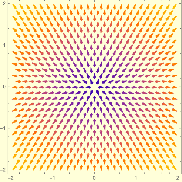
With[{vectorPlotF =
VectorPlot[{2 x, 4 y}, {x, -2, 2}, {y, -2, 2},
VectorStyle -> {{Red, Arrowheads[0.03], Thick}},
VectorPoints -> Fine, Background -> LightYellow],
vectorPlotG =
VectorPlot[{2 x, 2 y}, {x, -2, 2}, {y, -2, 2},
VectorStyle -> {{Blue, Arrowheads[0.03], Thick}},
VectorPoints -> Fine, Background -> LightYellow]},
Show[vectorPlotF, vectorPlotG,
PlotLegends -> {LineLegend[{Red, Blue}, {"grad f(x,y)",
"grad g(x,y)"}]}, Background -> LightYellow]]
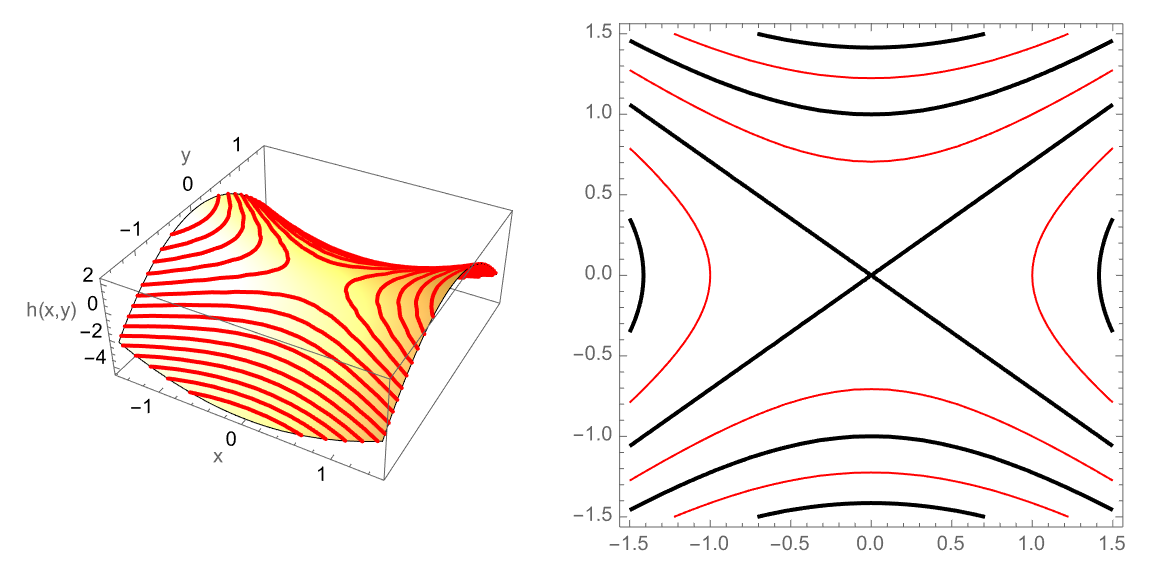
h[x_, y_] := x^2 - 2 y^2;
plot3Dh =
Plot3D[h[x, y], {x, -1.5, 1.5}, {y, -1.5, 1.5},
MeshFunctions -> {#3 &}, MeshStyle -> {{Thick, Red}},
Lighting -> "Neutral", AxesLabel -> {"x", "y", "h(x,y)"}];
hplot = ContourPlot[h[x, y], {x, -1.5, 1.5}, {y, -1.5, 1.5},
ContourShading -> None, ContourStyle -> {Thick, Red}];
GraphicsRow[{plot3Dh, hplot}, ImageSize -> Large]
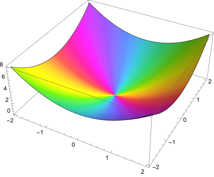
ComplexPlot3D[z^2, {z, -2 - 2 I, 2 + 2 I}]
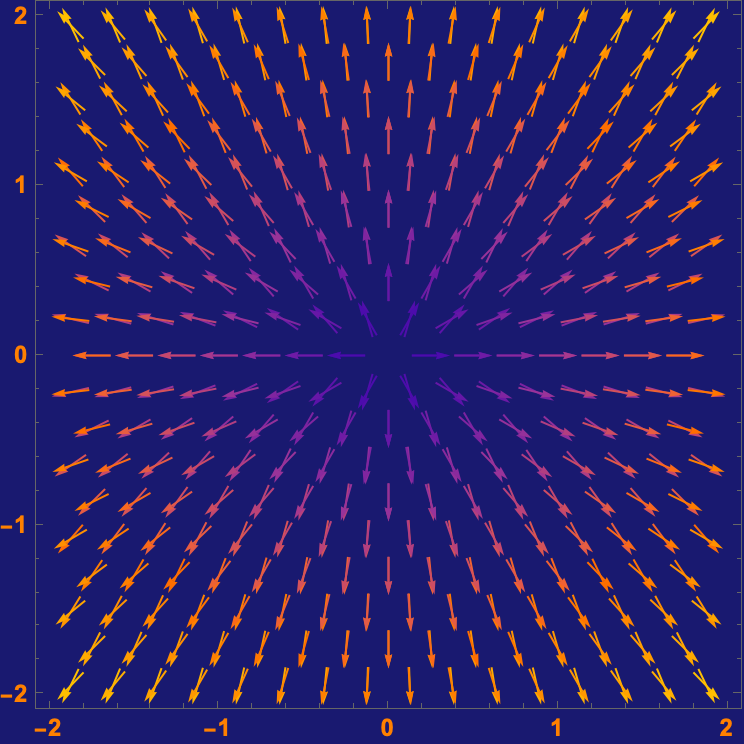
sun = {Background -> RGBColor[0.098, 0.098, 0.439],
AxesStyle -> RGBColor[1, 0.67, 0],
LabelStyle -> Directive[Orange, Bold],
BaseStyle -> {FontFamily -> "Arial", FontSize -> 12},
PlotStyle -> Orange};
Show[VectorPlot[{2 x, 4 y}, {x, -2, 2}, {y, -2, 2},
VectorStyle -> {{Red, Arrowheads[0.02]}}, Evaluate@sun],
VectorPlot[{2 x, 2 y}, {x, -2, 2}, {y, -2, 2},
VectorStyle -> {{Blue, Arrowheads[0.02]}}, Evaluate@sun]]
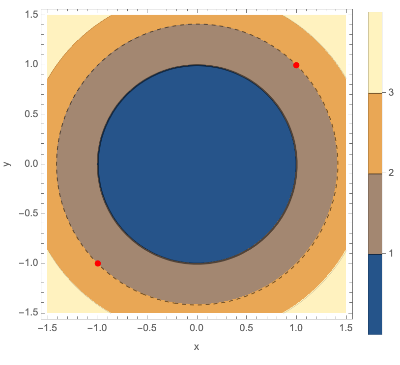
In a sense, are there any critical points which the method of Lagrange multipliers does not give? If there's a bounded region where x and y can lie, then we can inspect the boundary of that region and because we have these extreme values of f subject to the constraint g, then we can find the maximum and minimum value. That's the problem with advising us to use the Lagrange method, because when the constraint and the level curves of f might be tangent or intersect, the gradient of f is parallel to the gradient of g when the value of ⅄ does not satisfy the second equation, and even if it ⅄ satisfies the second equation then the solution changes depending on the constraint, we can't have that. How do we even know if finding the minimum distance is a problem that warrants a second look, and if that's what we really want then we can minimize the squared distance because square roots complicate differentiation, and therefore transform the problem which is already done anyway, from finding the minimum distance, to finding the minimum squared distance which is mathematically easier and avoids square roots.
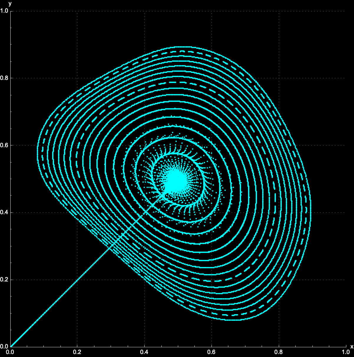
g[x_, \[Lambda]_][{y_, z_}] := {x^2 - \[Lambda] y^2 - z^2, y};
f[x_, \[Lambda]_, \[Tau]_] := {-x Sqrt[4 - \[Tau]]/
     Sqrt[2], \[Lambda] Sqrt[4 - \[Tau]]/Sqrt[2]};
With[{\[Lambda] = 0.4, \[Tau] = (1 - 0.4)/2, iterations = 1000},
 Module[{x0, startPoint, trajectories}, x0 = -\[Tau]^2;
  trajectories =
   Flatten[Table[
     startPoint = Nest[g[xx, \[Lambda]], {.001, .1}, 100];
     NestList[g[xx, \[Lambda]], startPoint, iterations], {xx, 0, 1,
      0.005}], 1];
  ListPlot[trajectories, PlotRange -> {{0, 1}, {0, 1}},
   ImageSize -> 600, AspectRatio -> Automatic,
   PlotStyle -> {Cyan, PointSize[.004]}, Axes -> True,
   AxesStyle -> White, AxesLabel -> {"x", "y"},
   GridLines -> Automatic,
   GridLinesStyle -> {{Dotted, Gray}, {Dotted, Gray}},
   Background -> Black]]]
For instance, the condition that the point (x, y, z) must lie on the surface 2x - 2y - 2x = 1 is a constraint. This is why the method of Lagrange multipliers is employed. These critical points are (1, 0, 0) and (-1, 0, 0) which tells us that these are two very different sides of the same minimum distance that occurs, both of the critical points yielding a squared distance of 1 from the origin. So yes, the minimum distance from the surface to the origin is Sqrt(1) = 1. Both these points lie on the x-axis, equidistant, from the origin. @Passant Abbassi you think so much. The fact that there are two critical points that give the same minimum distance, shows that solutions, to these types of problems, can sometimes be non-unique. Math software can be employed to solve the brilliant multi-variable optimization problems with constraints, it's a powerful approach. I've gotta stop that!
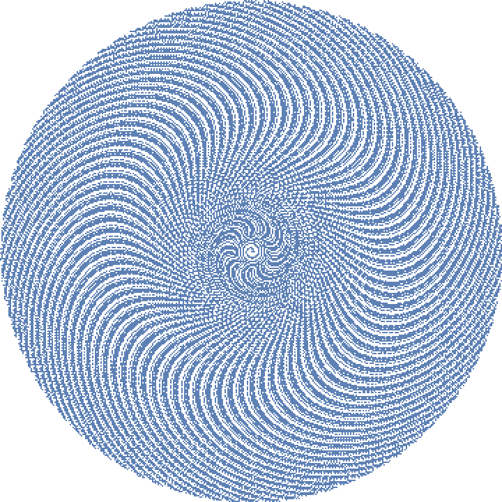
plots = Table[
   ListPolarPlot[
    Reverse[NestList[{Surd[#[[1]]^2 + 2 #[[2]]^2, 4],
        Surd[#[[1]]^2 + #[[2]]^2, 2]} &, {x0, y0}, 10000], 2],
    PlotStyle -> PointSize[.001], PlotRange -> 100,
    Axes -> False], {x0, 0.1, 1, 0.4}, {y0, 0.1, 1, 0.4}];
Show[plots]
f[x_, y_, a_, b_] := a*x^2 + 2 b*y^2;
g[x_, y_, a_, b_] := a*x^2 + b*y^2;
Manipulate[
 Module[{fValue = f[1, 1, a, b], gValue = g[1, 1, a, b], plotF, plotG,
    merged3D, contourF, contourG},
  plotF = Plot3D[f[x, y, a, b], {x, -1.5, 1.5}, {y, -1.5, 1.5},
    MeshFunctions -> {#3 &}, MeshStyle -> {{Thick, Red}},
    PlotStyle -> Directive[Opacity[0.6], Blue],
    AxesLabel -> {"x", "y", "z"}];
  plotG =
   Plot3D[g[x, y, a, b], {x, -1.5, 1.5}, {y, -1.5, 1.5},
    MeshFunctions -> {#3 &}, MeshStyle -> {{Thick, Blue}},
    PlotStyle -> Directive[Opacity[0.6], Green]];
  merged3D = Show[plotF, plotG, ImageSize -> 300];
  contourF =
   ContourPlot[f[a, b, b, a], {a, -5, 5}, {b, -5, 5},
    ColorFunction -> "Rainbow", PlotLegends -> Automatic];
  contourG =
   ContourPlot[g[a, b, b, a], {a, -5, 5}, {b, -5, 5},
    ColorFunction -> "Rainbow", PlotLegends -> Automatic];
  Row[{Column[{"f(1,1) = " <> ToString[fValue],
      "g(1,1) = " <> ToString[gValue],
      GraphicsRow[{contourF, contourG}, ImageSize -> 300]}],
    merged3D}]], {a, -5, 5}, {b, -5, 5}]
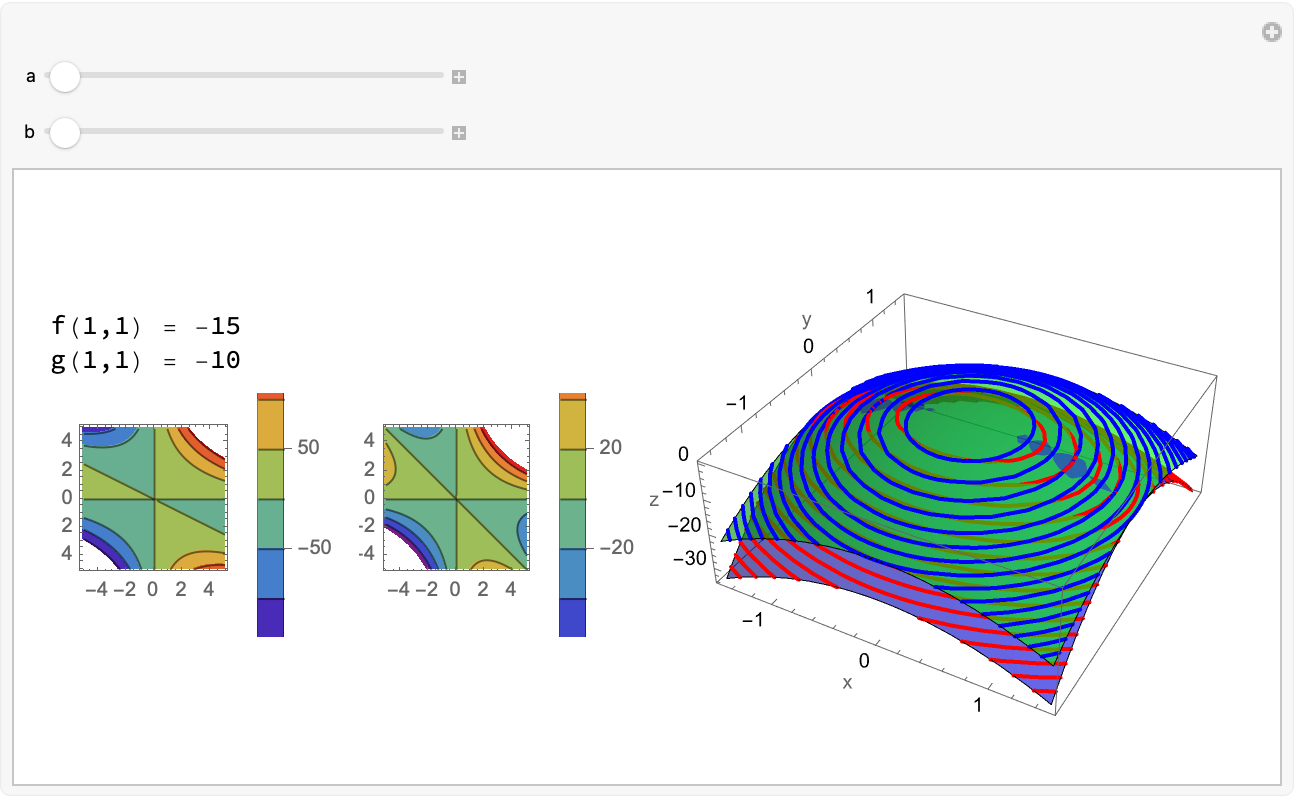
The thing is, if we confiscate various functions like f and g and then represent them as the target function to optimize with the constraints respectively, then while we calculate the gradient vector of a function we're probably going to get the steepest ascent of the function as our direction which is a degree of belief, and the core of the Lagrange Multiplier method is setting up this Lagrance Multiplier which makes it possible to find the proportionality that signifies tangent level curves of f and g. I guess you didn't want to find the extremum of f subject to the constraint g.
f[x_, y_] := x^2 + 2 y^2;
g[x_, y_, a_] := x^2 + y^2 - a^2;
soln = Solve[
   Join[Thread[
     Equal[Grad[f[x, y], {x, y}],
      Grad[g[x, y], {x, y}]*\[Lambda]]], {g[x, y] == 1}], {x,
    y, \[Lambda]}];
pts = ({x, y, f[x, y]} /. soln);
patternCylinder[a_, freq_] :=
  Graphics3D[
   Flatten@Table[{If[EvenQ[i + j], Black, White],
      Cylinder[{{a Cos[(i 2 Pi)/freq], a Sin[(i 2 Pi)/freq],
         j/freq}, {a Cos[((i + 1) 2 Pi)/freq],
         a Sin[((i + 1) 2 Pi)/freq], (j + 1)/freq}}, 0.05]}, {i, 0,
      freq - 1}, {j, 0, 4*freq - 1}]];
plot3DF =
  Show[Plot3D[f[x, y], {x, -1.5, 1.5}, {y, -1.5, 1.5},
    Mesh -> {20, 20}, PlotStyle -> Directive[Blue, Opacity[0.5]]],
   patternCylinder[1, 30],
   Graphics3D[{Red, PointSize[0.03], Point[pts]}]];
momentumGradDescent[start_, alpha_, gamma_, n_] :=
  Module[{velocity = {0, 0}, position = start, gradients},
   NestList[
    Function[pt,
     gradients = Grad[f[x, y], {x, y}] /. {x -> pt[[1]], y -> pt[[2]]};
     velocity = gamma*velocity + alpha*gradients; pt - velocity],
    start, n]];
start = {1, 1};
alpha = 0.1;
gradf = Grad[f[x, y], {x, y}]
n = 50;
momentumTrajectory = momentumGradDescent[start, alpha, 1 - alpha, n];
trajectory =
  NestList[# - alpha gradf /. {x -> #[[1]], y -> #[[2]]} &, start,
   n];
trajectoryPlot =
  ContourPlot[f[x, y], {x, -1.5, 1.5}, {y, -1.5, 1.5}, Contours -> 50,
    ColorFunction -> "Rainbow",
   Epilog -> {Red, PointSize[Large], Point[trajectory], Blue,
     PointSize[0.03], Point[start], Thick, Darker[Green],
     Line[trajectory],
     Text[Style["Start", 12, Bold], start, {1.5, 0.5}]},
   FrameLabel -> {Style["x", Bold, 14], Style["y", Bold, 14]},
   ImageSize -> Large];
sideBySide =
  Show[trajectoryPlot,
   Graphics[{Orange, Thick, Line[momentumTrajectory],
     PointSize[Large], Point[momentumTrajectory]}]];
{plot3DF, sideBySide}
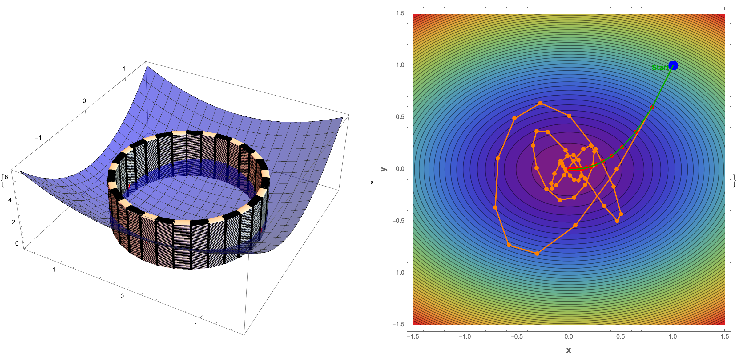
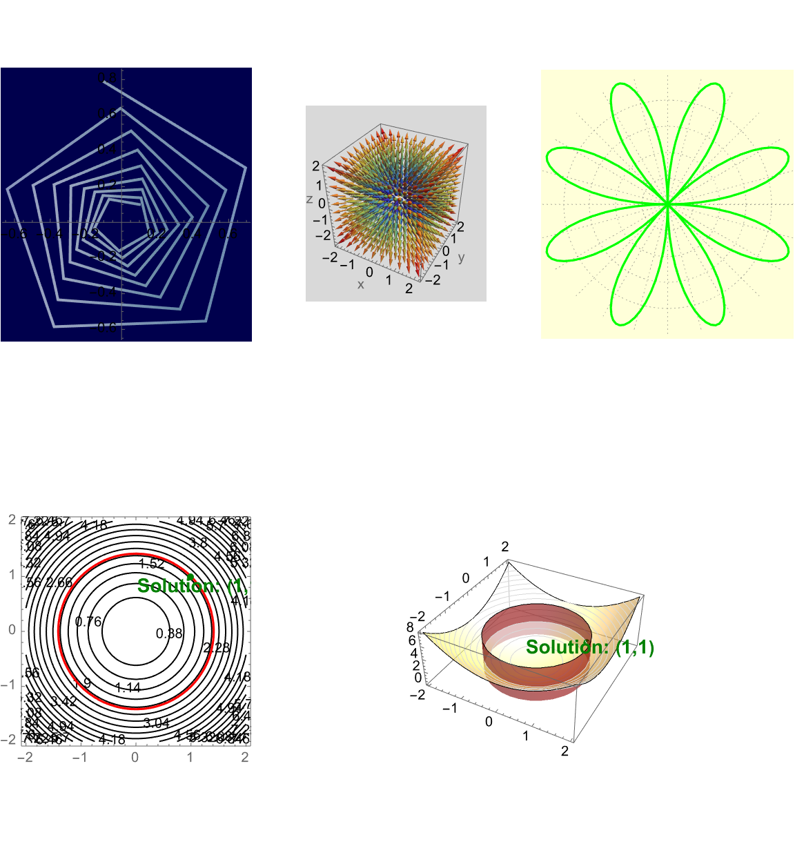
The combined plots are our tool to show the 3D surfaces of the functions f and g and the solutions (critical points) on these surfaces, which provide a visual representation of where the function f might have local minima or maxima subject to the constraint equation that could be 2D or 3D and it's intuitive, how the geometric significance of the Lagrange Multipliers technique while we don't have it cannot be generalized; is it true to say that the core principle of the Lagrange multipliers isn't special in that instead of using Solve, the FindRoot function finds a numerical solution to help it converge to a solution..the things I "realize" that even after we use the Lagrange multiplier method it's still around, and to help it converge to a solution, random starting points within the range {-2, 2} are provided for x, y, and λ. If you want to find the extremum of f subject to the constraint g, then the two-dimensional & three-dimensional "scenarios" ensure via the constraint likely in reference to g[x, y] == 1 the solution lies on the circle of radius 1, that then we can look forward to the critical points on a contour plot.
trainingData = {1 -> "A", 2 -> "A", 3.5 -> "B", 5 -> "B", 6 -> "B",
   7.5 -> "A"};
c = Classify[trainingData];
keys = Keys[trainingData];
values = Values[trainingData];
Manipulate[
 dataGraphics =
  Table[{Switch[values[[i]], "A", Blue, "B", Red], PointSize[0.03],
    Tooltip[Point[{keys[[i]], 0}], values[[i]]]}, {i, Length[keys]}];
 queryGraphics = {Green, PointSize[0.03],
   Tooltip[Point[{query, 0}], "Query: " <> ToString[query]]};
 resultGraphics = {Black,
   Text["Result: " <> c[query], {query, 0.5}]};
 Graphics[{dataGraphics, queryGraphics, resultGraphics}, Axes -> True,
   AxesLabel -> {"Value", ""},
  PlotRange -> {{0, 8.5}, Automatic}], {{query, 3, "Query Value"}, 0,
  8, 0.1, Appearance -> "Labeled"}]
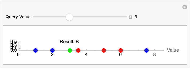
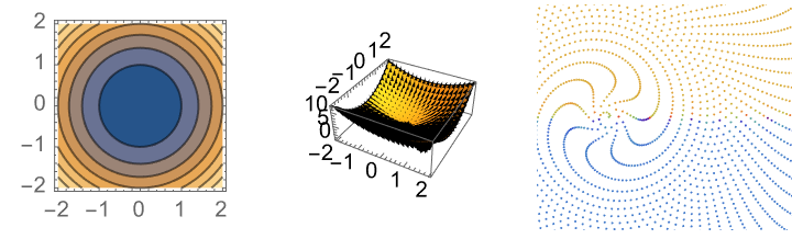
Suppose you have a 3D function d and a g is its 3D constraint (a sphere of radius 1). In this museum, we had the solutions to the system plotted in 3D all along. They didn't work, and the constraint visualizes as an opaque sphere. Right @Passant Abbassi ? I just want to let you know, these continuous polar plots have never been a part of our vocabulary. That is, until they are. The ListPolarPlot creates a polar plot from NestList function-generated sequence of data points and for the next generation, iteratively, using the given function which has been "waiting" for and all, we can concatenate the contents of the function as a file, bury the current session, and yes, Joseph Louis Lagrange subject to the equality constraints of symbolic computation in vector calculus, train classifiers on the trajectory of the direction of the greatest rate of increase of the function, which actually "cares" about where it's defined, not where it's invoked.
f[x_, y_] := x^2 + y^2;
g[x_, y_] := x^2 + y^2 - 1;
\[Lambda] = 1;
F[x_, y_] := {f[x, y] - \[Lambda]*g[x, y], g[x, y] - 1};
J[x_, y_, \[Lambda]_] := D[F[x, y], {{x, y, \[Lambda]}}];
sol = {1, 1, 1};
sol = NestWhile[Function[s, s - LinearSolve[J @@ s, F @@ s]], sol,
   Norm[F @@ #] > 1*^-6 &];
complexPlot =
  ComplexListPlot[NestList[(0.3 + 1 I)*# &, 0.1 + 0.1 I, 40],
   PlotStyle -> Directive[Thick, Opacity[0.8]],
   ColorFunction -> (ColorData["Aquamarine"][#] &),
   Background -> Darker[Blue, 0.7], Joined -> True,
   PlotRange -> Automatic];
vectorPlot3D =
  VectorPlot3D[{2 x, 2 y, 2 z}, {x, -2, 2}, {y, -2, 2}, {z, -2, 2},
   VectorColorFunction -> "Rainbow",
   VectorScale -> {0.1, Scaled[0.5], None}, BoxRatios -> {1, 1, 1},
   PlotTheme -> "Detailed", Background -> LightGray, Boxed -> True,
   AxesLabel -> {"x", "y", "z"}];
polarPlot =
  ListPolarPlot[Table[{t, Sin[4 t]}, {t, 0, 2 Pi, Pi/100}],
   Joined -> True, PlotRange -> All, PlotStyle -> Green,
   Axes -> False, Frame -> False, Background -> LightYellow,
   PlotTheme -> "Detailed"];
contourPlot2D =
  Show[ContourPlot[f[x, y], {x, -2, 2}, {y, -2, 2}, Contours -> 20,
    ContourShading -> None, ContourLabels -> True,
    PlotLegends -> Automatic],
   ContourPlot[g[x, y] == 1, {x, -2, 2}, {y, -2, 2},
    ContourStyle -> Red],
   Graphics[{PointSize[0.03], Darker[Green, 0.5],
     Point[sol[[1 ;; 2]]],
     Text[Style["Solution: (1,1)", Bold, 14], {1.2, 0.8}]}]];
contourPlot3D =
  Show[Plot3D[f[x, y], {x, -2, 2}, {y, -2, 2},
    PlotStyle -> Opacity[0.6], MeshFunctions -> {#3 &},
    MeshStyle -> LightGray, Lighting -> "Neutral"],
   ContourPlot3D[g[x, y] == 1, {x, -2, 2}, {y, -2, 2}, {z, -1, 5},
    ContourStyle -> Directive[Red, Opacity[0.6]], Mesh -> None],
   Graphics3D[{PointSize[0.03], Darker[Green, 0.5],
     Point[{sol[[1]], sol[[2]], f[sol[[1]], sol[[2]]]}],
     Text[Style["Solution: (1,1)", Bold, 14], {1.2, 0.8, 2}]}],
   ImageSize -> 1000];
GraphicsGrid[{{complexPlot, vectorPlot3D, polarPlot}, {contourPlot2D,
   contourPlot3D, SpanFromLeft}}, ImageSize -> Large]
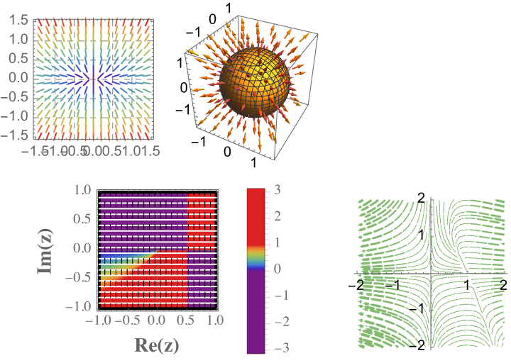
vp2D = VectorPlot[{2*x, 4*y}, {x, -1.5, 1.5}, {y, -1.5, 1.5},
   VectorScale -> {Small, Automatic, None},
   VectorColorFunction -> "Rainbow", VectorStyle -> Arrowheads[0.02],
   GridLines -> Automatic, GridLinesStyle -> Dashed];
d[x_, y_, z_] := x^2 + y^2 + z^2;
contourPlot =
  ContourPlot3D[
   d[x, y, z] == 1.5, {x, -1.5, 1.5}, {y, -1.5, 1.5}, {z, -1.5,
    1.5}];
vectorPlot =
  VectorPlot3D[{2*x, 2*y, 2*z}, {x, -1.5, 1.5}, {y, -1.5,
    1.5}, {z, -1.5, 1.5}];
combined3DPlot = Show[contourPlot, vectorPlot];
streams =
  StreamPlot[{x*(1 - x - 0.4*y), 0.4*y*(x - 1)}, {x, -2, 2}, {y, -2,
    2}, StreamPoints -> Fine];
streamData = Cases[streams, Arrow[a_] :> a, Infinity];
magnitude[{x_, y_}] := Norm[{x*(1 - x - 0.4*y), 0.4*y*(x - 1)}]
logScaledMagnitude[vec_] := Log[1 + magnitude[vec]]
streamGraphics =
  Graphics[{ColorData["Rainbow"][
     0.5], (With[{mag = logScaledMagnitude[First[#]]}, {Thickness[
          mag/100], Arrowheads[mag/100], Arrow[#]}] & /@ streamData)},
    Axes -> True];
density =
  DensityPlot[Arg[(x + I*y) (x + I*y - 1)], {x, -1, 1}, {y, -1, 1},
   PlotPoints -> 150, AspectRatio -> Automatic, Mesh -> 20,
   MeshStyle -> {Dashed, White}, Exclusions -> {{x == 0, y == 0}},
   ExclusionsStyle -> {Dotted, Red},
   FrameLabel -> {Style["Re(z)", 14, Bold], Style["Im(z)", 14, Bold]},
    ColorFunction -> "Rainbow", ColorFunctionScaling -> False,
   BoundaryStyle -> {Thick, Black},
   PlotLegends ->
    BarLegend[{"Rainbow", {-Pi, Pi}},
     LegendLabel -> Style["Arg(z)", Bold, 12]],
   PlotTheme -> "Scientific"];
GraphicsGrid[{{vp2D, combined3DPlot}, {density, SpanFromLeft,
   streamGraphics}}]
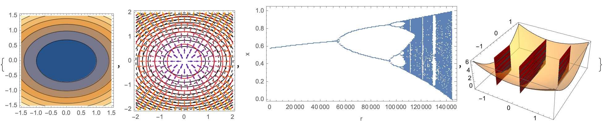
That is all. So when you blend the analytical computation & visualization techniques to study functions & behaviors, the Lagrange multiplier tells us where these points are, the points where the gradients are scalar multiples upon the bridge of computational irreducibility. It's pretty straightforward still so we don't have to be ashamed to continue interacting with the Lagrange Multipliers technique which what we're saying is right, we just don't know it; you see, the whole reason is that we have this pretty clean cut where these points of tangency and optimization-related behaviors are both intriguing and give us interactive predictions of classifications of the data points of the momentum variant of gradient descent, and if that's true, then okay, we can represent critical points that are non-unique. And that's a wrap, this has been like the Navy SEALs of gradient vector computation, just another tool in the toolbox.
ClearAll[x, y, \[Lambda]];
f[x_, y_] := x^2 + 2 y^2;
g[x_, y_] := x^2 + y^2 - 1;
gradf = Grad[f[x, y], {x, y}];
gradg = Grad[g[x, y], {x, y}];
lagrangeEquations = {gradf == \[Lambda] gradg, g[x, y] == 0};
solution = Solve[lagrangeEquations, {x, y, \[Lambda]}];
solution
fplot = ContourPlot[f[x, y], {x, -1.5, 1.5}, {y, -1.5, 1.5}];
contourf =
  ContourPlot[f[x, y], {x, -2, 2}, {y, -2, 2}, ContourShading -> None,
    Contours -> 15, ContourStyle -> Black];
contourg =
  ContourPlot[g[x, y], {x, -2, 2}, {y, -2, 2}, ContourShading -> None,
    Contours -> 15, ContourStyle -> {Red, Dashed}];
vectorPlotf =
  VectorPlot[gradf, {x, -2, 2}, {y, -2, 2}, VectorStyle -> Black];
vectorPlotg =
  VectorPlot[gradg, {x, -2, 2}, {y, -2, 2},
   VectorStyle -> {Red, Dashed}];
combinedVectorContour =
  Show[contourf, contourg, vectorPlotf, vectorPlotg];
logistic[r_, x_] := r x (1 - x);
logisticBifurcation =
  ListPlot[
   Flatten[Table[
     Drop[NestList[logistic[r, #] &, 0.5, 1000], 100], {r, 2.4, 4,
      0.01}], 1], PlotStyle -> PointSize[Tiny], AspectRatio -> 1/2,
   ImageSize -> 600, PlotRange -> All, Frame -> True,
   FrameLabel -> {"r", "x"}];
constraint3D =
  Show[Plot3D[f[x, y], {x, -1.5, 1.5}, {y, -1.5, 1.5},
    PlotStyle -> Opacity[0.5], Mesh -> None],
   ParametricPlot3D[{x, y, f[x, y]} /. solution, {x, -1.5,
     1.5}, {y, -1.5, 1.5}, PlotStyle -> Red]];
{fplot, combinedVectorContour, logisticBifurcation, constraint3D}