Stochastic pathfinding, we can spotlight the winning path by fading out all other trajectories as soon as a particle reaches the exit, without any magic wand or telepathy needed. Telepathy, was something people generally believed was right around the corner. It was a different scientific and intellectual time. It seemed inconceivable that you could just type to a computer and it would behave in a human-like way. Indeed, for a long time that seemed inconceivable until it turned out in 2022 that Large Language Models could produce pretty plausible natural language text. How human-like is it? Alan Turing's test is--you talk to the thing does it seem like there is a human there or not? That's a weird kind of test, there are humans you can talk to but it's certainly not something which one can immediately identify as being like itself. The question is, people in past years connect Wolfram Alpha to a Turing test, test type of system..which system has Wolfram Alpha connected to it and which doesn't? If it answers them, it's a machine. If it can't answer them, it might be a human. Below you will find nothing but an extension to Brownian Motion Maze Solving (based on "The Dumbest Way To Solve A Maze") that builds on its core idea of solving a maze with Brownian motion--but now with a twist. Once the maze is solved (that is, when one particle reaches the exit), the simulation automatically makes all the other paths transparent, spotlighting the winning route. For us, this extension not only enhances the flavor of our visual clarity but also does reinforce the metaphor of a "lucky" path emerging from a sea of randomness.
dims = {8, 8, 8};
mazeGraph = GridGraph[dims, EdgeWeight -> (_ :> RandomReal[])];
spanningTree = FindSpanningTree[mazeGraph];
graphEdges = EdgeList[spanningTree];
vertexList = VertexList[mazeGraph];
nodeCoords =
  AssociationThread[
   vertexList ->
    Map[Function[
      i, {Mod[i - 1, dims[[1]]] + 1,
       Mod[Floor[(i - 1)/dims[[1]]], dims[[2]]] + 1,
       Floor[(i - 1)/(dims[[1]]*dims[[2]])] + 1}], vertexList]];
pathSegments = Line[Lookup[nodeCoords, #]] & /@ graphEdges;
hallwayThickness = 0.3;
mazeRegion =
  RegionUnion[
   RegionDilation[DiscretizeGraphics[Graphics3D[pathSegments]],
    Ball[{0, 0, 0}, hallwayThickness]],
   Cuboid[{hallwayThickness, hallwayThickness, hallwayThickness},
    dims + 1 - hallwayThickness]];
particleCount = 5;
initPos = {1.5, 1.5, 1.5};
maxSteps = 1000;
timeStep = 1;
correlationMatrix = {{1, 0.8, 0.5}, {0.8, 1, 0.6}, {0.5, 0.6, 1}};
chol = CholeskyDecomposition[correlationMatrix];
simulateParticles[] :=
  Module[{positions, velocities, paths, inMazeQ},
   inMazeQ = RegionMember[mazeRegion];
   positions = ConstantArray[initPos, particleCount];
   paths = Table[ConstantArray[initPos, maxSteps], {particleCount}];
   Do[velocities =
     Transpose[
      chol . Transpose[
        RandomVariate[
         NormalDistribution[0, 0.15], {particleCount, 3}]]];
    positions += velocities*timeStep;
    positions =
     Table[If[inMazeQ[positions[[i]]], positions[[i]],
       positions[[i]] - velocities[[i]]*timeStep], {i, 1,
       particleCount}];
    paths[[All, i]] = positions, {i, 2, maxSteps}];
   paths];
particlePaths = simulateParticles[];
endPoint = dims;
winningData =
  Table[With[{winStep =
      FirstPosition[particlePaths[[i]],
       pos_ /; And @@ Thread[pos > 8]]},
    If[winStep === Missing["NotFound"],
     Nothing, {i, winStep[[1]]}]], {i, particleCount}];
If[Length[winningData] > 0, {winner, winningStep} =
   First[SortBy[winningData, Last]], winner = None;
  winningStep = maxSteps];
Manipulate[
 Graphics3D[{{Directive[Purple, Opacity[0.3]],
    Polygon[{{8, 0, 0}, {8, dims[[2]] + 1, 0}, {8, dims[[2]] + 1,
       dims[[3]] + 1}, {8, 0, dims[[3]] + 1}}]}, {Opacity[0.2,
     LightBlue], mazeRegion},
   If[winner =!= None &&
     step >= winningStep, {{Directive[Thick, Black],
      Tube[particlePaths[[winner, ;; step]], 0.1]}, {Green,
      Text[Style[
        "Winner " <> ToString[winner] <> " @ step " <>
         ToString[winningStep] <> " at " <>
         ToString[particlePaths[[winner, winningStep]]], Bold, 14],
       particlePaths[[winner, winningStep]]]},
     Table[{Opacity[0.2], Tube[particlePaths[[n, ;; step]], 0.05],
       Sphere[particlePaths[[n, step]], 0.1]}, {n,
       DeleteCases[Range[particleCount], winner]}]},
    Table[{ColorData["Rainbow", n/particleCount],
      Tube[particlePaths[[n, ;; step]], 0.05],
      Sphere[particlePaths[[n, step]], 0.1]}, {n,
      particleCount}]], {Red, Sphere[initPos, 0.2]}, {Black,
    Text[Style["End", Bold, 14], endPoint + {0, 0, 0.5}]}},
  PlotRange -> {{0, dims[[1]] + 1}, {0, dims[[2]] + 1}, {0,
     dims[[3]] + 1}}, Boxed -> True, Lighting -> "Neutral",
  ImageSize -> 600, SphericalRegion -> True,
  RotationAction -> "Clip"], {step, 1, maxSteps,
  1}, {{correlationMatrix, correlationMatrix, "Correlation Matrix"},
  InputField[#, ImageSize -> Small] &},
 TrackedSymbols :> {step, correlationMatrix},
 SynchronousUpdating -> False]
Extending the Brownian Motion Maze Simulation: Focus on the Winning Path
In our previous work we showed how particles wandering via Brownian motion eventually find their way out of a maze. Today, we add a tangible twist: at the very moment when a particle reaches the exit, every other particle's path fades away. This approach mirrors real-world decision making--once the optimal path is identified, all other alternatives lose their relevance. What's new? Well, it's quite simple. In our Graphics3D visualization (within a Manipulate construct), we adjust the rendering logic so that once the winning condition is met (i.e. when a particle's position exceeds the purple glowing exit threshold), the paths of all non-winning particles are drawn with "minimalistic" opacity. The winning path, on the other hand, "provides" a bird's eye view, a computational windowsill onto which we can reconstruct the voxels of which route led out of the maze. This not only builds the visual narrative by clearly isolating the successful path but also builds the scaffolding of the metaphor: amid many random journeys, one optimal path emerges from the noise.
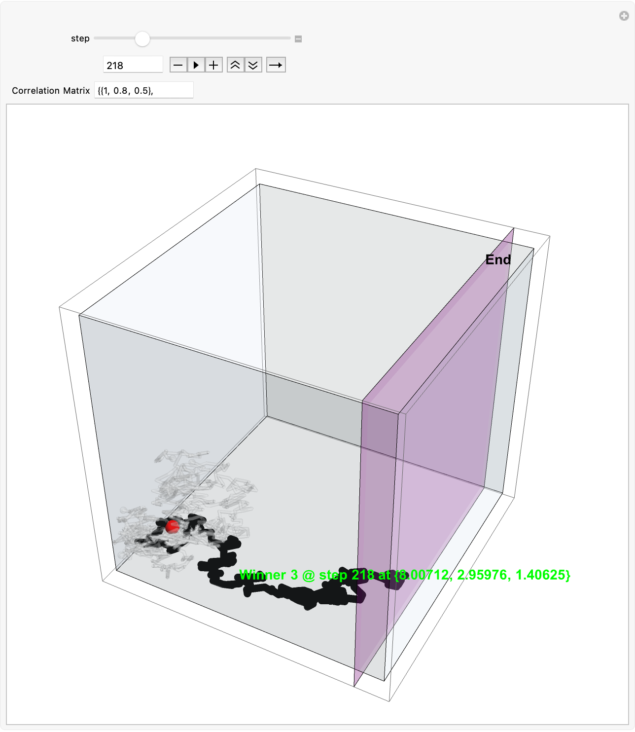
Why does this matter? Because we remove unnecessary visual clutter and make the result immediately apparent. We could easily just sit down and draw out simulations where a "best" solution exists and needs to be spotlighted or we could draw the many competing paths and add a visual cue that emphasizes the success among randomness--a small change that can make a big difference in our understanding of complex stochastic systems. Every particle can be conceived of as an independent contractor and with the right visual signal we can set the flag winner and record the winningStep step at which it happens, and revamp all competing paths so we don't have to search. But like they say, give me some computational framework and we can articulate any idea..even if it's in Python or COBOL. Even before the web one could search, there were online database systems that would search it's kind of like how Bluetooth could be pretty useful...a lot of the time we use the power of teamwork and the computation, the graphical capabilities that we've got when we're cracking these chestnuts..what if something new came along...and we didn't get all the simulations represented that we wanted to represent within the Brownian motion that we are portraying, which describes the random movement of particles suspended in a fluid, like graphene. It's a fundamental concept and it honestly looks like the soot, the thermal motion of molecules that, in the context of maze solving, might allow us to repurpose this computational metaphor. We should get a Nobel Prize for what we did with this maze it's the greatest path of all time through this complex structure...where we don't just mesh all these particles together, we can simulate and redo random steps of particles until one reaches an exit point. And this is what we're missing out on, whenever we solve a maze.
dims = {8, 4};
hallwayThickness = 0.8;
ballCount = 1000;
spanningTree = FindSpanningTree[
   GridGraph[dims,
    EdgeWeight -> {_ :> RandomReal[]}]
   ];
outerRegion =
  Rectangle[{1, 1} - 1 + hallwayThickness, Reverse[dims] + 1];
wallsRegion = RegionDifference[
   RegionDifference[
    Rectangle[{1, 1} - 1 + hallwayThickness, Reverse[dims] + 1],
    RegionDilation[
     DiscretizeGraphics[
      Line[GraphEmbedding[spanningTree][[#]]] & /@
       List @@@ EdgeList[spanningTree]],
     Rectangle[{0, 0}, {1, 1}*hallwayThickness]]],
   Rectangle[
    {dims[[2]], hallwayThickness},
    {dims[[2]], 0} + {hallwayThickness, 1}
    ]
   ];
wallMember = RegionMember[wallsRegion];
mazeMember = RegionMember[outerRegion];
initPs = {1 + hallwayThickness/2, dims[[1]] + hallwayThickness/2};
magneticField = -0.05;
positionSeries = Module[{ps, vs, magnetEffect},
   Monitor[ps = ConstantArray[initPs, ballCount];
    Reap[Sow[ps];
      While[And @@ mazeMember[ps],
       vs = RandomPoint[Circle[], ballCount]*0.1;
       magnetEffect = If[First[#] <= (1 + hallwayThickness/2),
           {0, magneticField},
           {0, 0}] & /@ ps;
       ps = MapThread[
         If[wallMember[#1 + #2 + #3],
           #1, #1 + #2 + #3] &,
         {ps, vs, magnetEffect}];
       Sow[ps]]
      ][[2, 1]],
    Graphics[
     {wallsRegion, Orange, PointSize[0.025], Point[ps]},
     ImageSize -> Large]]];
winningIndex =
 FirstPosition[mazeMember@Last@positionSeries, False][[1]]
Graphics[{
  wallsRegion,
  Orange,
  Line[positionSeries[[All, winningIndex]]]
  }, ImageSize -> Large]
Manipulate[Graphics[{wallsRegion,
   If[i > Length[positionSeries]*2/3,
    {Red, Thick, Circle[positionSeries[[i, winningIndex]], 0.01],
     Thin, Blue, Line[positionSeries[[All, winningIndex]]]},
    {}],
   Orange,
   PointSize[Medium],
   Point[positionSeries[[i]]]},
  ImageSize -> Large],
 {i, 1, Length[positionSeries], 1}
 ]
ballMaxDistances =
  Max /@ Total[(Threaded[initPs] -
       Transpose[positionSeries])^2, {3}];
ballDistanceRanking = Ordering[ballMaxDistances];
Manipulate[
 Graphics[{wallsRegion,
   Orange,
   Line[positionSeries[[All, ballDistanceRanking[[n]]]]]
   }, ImageSize -> Large],
 {n, 1, ballCount, 1}]
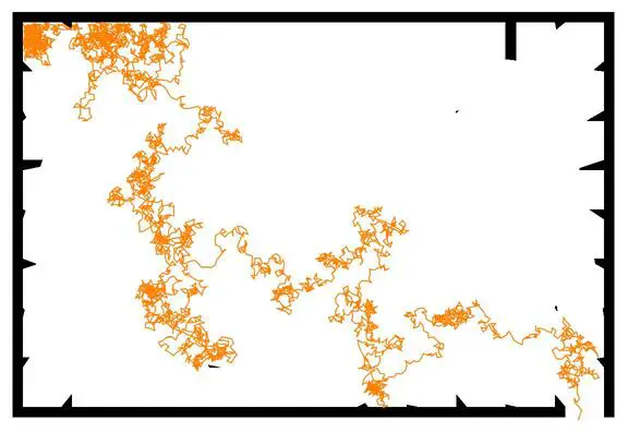
For the ten million degrees centigrade plasma that has enough particles that they want to undergo fusion, even if you can contain it with some kind of magnetic field...you can reflect the natural process of scientific phenomena including diffusion and pathfinding within this magnetic field, and because of the tree structure it's this maze that is generated without loops, directed and acyclic in that the possibility of a unique path between any two points is predetermined..in that simulation the Brownian motion exists within the confines of the maze walls, and if a particle intersects with a wall it reverses its direction across molecular space to avoid crossing into the wall, thus remaining within the valid paths of the maze...potentially we can Reap and Sow the path of each particle and effectively solve the maze and determine the first particle to reach the exit. It's a slow, steady progress that allows for real-time observation of particles' paths and their distances post-simulation...which is the first particle to reach the threshold beyond the exit? How does the simulation evolve across the time-lapse of the particles' positions or and the temporal progression of the simulation?
The metaphor of the pulled string means that even post-simulation the winning path can be optimized, yes vacuum tubes have been developed for many years...while the initial path found may be circuitous it can be refined to a more direct route..which is how we solve optimization problems like the unsupervised spectral clustering that occurs within a dishwasher, or the operations research that we do and I do, I suggest the statistical analysis that shows us the characteristics of the Brownian paths within the maze which might as well be 35 years old and that takes over the things we think about as opposed to say low-level programming languages, which putatively can in that case describe the incumbent characteristics of the Brownian paths within the maze. And that's why we've got this tiny little wheel of computational simulation that allows us to explore computational space to mimic and mirror the most intricate of things..like let's say we want to add padding to the side of a microscopic particle interaction, scenario card or add a table of contents to our model of particle dynamics? I think the collision detection and handling emphasizes the foundation of creativity in that assigning value to something like Bitcoin or mathematical axioms allows us to build our own Brownian motion simulation, a hangout where the question of whether or not we need to redo our underlying rules of particle interaction can be rewritten with a resounding yes, as this vast, interconnected Ruliad concept what with its hypergraphs making up the fabric of hyperspace; it proposes a discrete structure and in the simulation each particle's path through the maze, is discretely determined by the local interactions with the maze walls and other particles, which encapsulates the infrageometry of the Ruliad as a microcosm of the conservation laws when two particles collide - much like the molecules governed by collisions which are elastic...the kinetic energy of the particle system is conserved in this Newtonian cradle where the unpredictable nature of particle dynamics adheres to the physical laws that govern our universe.
dims = {10, 14};
hallwayThickness = 1;
ballCount = 100;
particleRadius = 0.05;
timeStep = 0.05;
baseOrange = RGBColor[1, 0.5, 0];
colors = Table[
   Lighter[baseOrange, RandomReal[{0, 0.5}]],
   {ballCount}];
initialPosition = {2 + hallwayThickness,
   dims[[2]] - hallwayThickness - 2};
positions = Table[initialPosition, {ballCount}];
velocities = RandomReal[{-1, 1}, {ballCount, 2}];
paths = Table[{}, {ballCount}];
generateDiagonal[start_, end_, count_] := Module[
   {
    dx = (end[[1]] - start[[1]])/count,
    dy = (end[[2]] - start[[2]])/count,
    step
    },
   step = Min[Abs[dx], Abs[dy]];
   Table[
    {
     {start[[1]] + i*dx, start[[2]] + i*dy},
     {start[[1]] + i*dx + step, start[[2]] + i*dy + step}
     },
    {i, 0, count - 1}]
   ];
wallCoordinates = {
   {{3, 3}, {7, 5}},
   {{2, 7}, {4, 9}},
   {{1.75, 0}, {2, 15}},
   {{9.25, 0}, {9.5, 15}},
   {{0, 13.25}, {11, 13.5}},
   {{0, 1.75}, {8.5, 2}}};
obstacles = Join[
   wallCoordinates,
   generateDiagonal[{8, 4}, {4, 10}, 10]
   ];
reflectBounceParticleWall[pos_, vel_, obstacles_] := Module[
   {newPos = pos, newVel = vel, reflect,
    minTimeStep = timeStep, xCollision, yCollision},
   reflect = False;
   xCollision = False;
   yCollision = False;
   Do[
    newPos = pos + vel*timeStep;
    newPosNew = pos + vel*2*timeStep;
    newPosNewPos = pos + vel*3*timeStep;
    If[(pos[[1]] >= obs[[1, 1]] && pos[[1]] <= obs[[2, 1]] &&
        pos[[2]] >= obs[[1, 2]] && pos[[2]] <= obs[[2, 2]]
       ) ||
      (newPos[[1]] >= obs[[1, 1]] && newPos[[1]] <= obs[[2, 1]] &&
        newPos[[2]] >= obs[[1, 2]] && newPos[[2]] <= obs[[2, 2]]
       ) ||
      (newPosNew[[1]] >= obs[[1, 1]] &&
        newPosNew[[1]] <= obs[[2, 1]] &&
        newPosNew[[2]] >= obs[[1, 2]] &&
        newPosNew[[2]] <= obs[[2, 2]]
       ) ||
      (newPosNewPos[[1]] >= obs[[1, 1]] &&
        newPosNewPos[[1]] <= obs[[2, 1]] &&
        newPosNewPos[[2]] >= obs[[1, 2]] &&
        newPosNewPos[[2]] <= obs[[2, 2]]),
     reflect = True;
     If[
      Abs[newPos[[1]] - obs[[1, 1]]] <= particleRadius ||
       Abs[newPos[[1]] - obs[[2, 1]]] <= particleRadius,
      xCollision = True
      ];
     If[
      Abs[newPos[[2]] - obs[[1, 2]]] <= particleRadius ||
       Abs[newPos[[2]] - obs[[2, 2]]] <= particleRadius,
      yCollision = True
      ];
     If[xCollision, newVel[[1]] = -vel[[1]]];
     If[yCollision, newVel[[2]] = -vel[[2]]];
     ],
    {obs, obstacles}
    ];
   If[reflect, newPos = pos - vel*timeStep];
   If[reflect, newPos += newVel*minTimeStep];
   {newPos, newVel}
   ];
updateGraph[positions_, velocities_] := Transpose[
   MapThread[
    reflectBounceParticleWall,
    {
     positions + velocities*timeStep,
     velocities,
     ConstantArray[obstacles, Length[positions]]
     }
    ]
   ];
onCollideHandle[positions_, velocities_] := Module[
   {newVelocities = velocities, angle,
    v1, v2, speed1, speed2},
   Do[
    If[i != j &&
      Norm[positions[[i]] - positions[[j]]] < 2*particleRadius,
     angle = RandomReal[{0, 2 Pi}]; speed1 = Norm[velocities[[i]]];
     speed2 = Norm[velocities[[j]]];
     v1 = speed1*{Cos[angle], Sin[angle]};
     v2 = speed2*{Cos[angle + Pi], Sin[angle + Pi]};
     newVelocities[[i]] = v2;
     newVelocities[[j]] = v1;
     ],
    {i, ballCount},
    {j, i + 1, ballCount}];
   newVelocities
   ];
stringRewritePath[positions_, paths_] :=
  MapThread[Append, {paths, positions}];
findFirstWinFirstTime[positions_, yThreshold_] := Module[
   {foundPosition = None},
   Do[
    If[positions[[i, 2]] <= yThreshold,
     foundPosition = i;
     Break[];],
    {i, Length[positions]}];
   foundPosition
   ];
winFirstTime = None;
positionSeries = Table[
   paths = stringRewritePath[positions, paths];
   If[winFirstTime === None,
    With[
     {win = findFirstWinFirstTime[positions, 1.5]},
     If[win =!= None, winFirstTime = win]
     ]
    ];
   velocities = onCollideHandle[positions, velocities];
   {positions, velocities} = updateGraph[positions, velocities];
   {positions, velocities, paths},
   {t, 0, 10, timeStep}
   ];
highlightPath[paths_, index_] := If[
   index =!= None && index <= Length[paths],
   {Thick, Purple, Line[paths[[index]]]},
   {}
   ];
pizzatoppings = ListAnimate[
   Table[
    Graphics[
     {
      highlightPath[paths, winFirstTime],
      Table[
       {colors[[i]], PointSize[Large],
        Point[positionSeries[[frame, 1, i]]]},
       {i, ballCount}
       ],
      Black,
      Rectangle[#1, #2] & @@@ obstacles
      },
     PlotRange -> {{0, dims[[1]] + 1}, {0, dims[[2]] + 1}},
     Frame -> True
     ],
    {frame, Length[positionSeries]}],
   AnimationRate -> 10
   ];
pizzatoppings
Does everybody who gets the flu, is there a higher probability of them getting this other thing later? The question of Brownian motion becomes a playground for testing theories of emergent properties like the trajectory of the paths of particles as an allegory for the process of discovery itself, whether homomorphic encryption on zero-knowledge, mathematically simplistic things can be understood. How can we understand the context of the behavior of the system of Brownian Motion Maze Solving which is the best maze solving..if you were wondering how the behavior of a system can be understood in the context of the observer's interaction with the system, the observer which witnesses and tracks the particles' movements, the observer (simulation) must have rules or assumptions that govern its interaction with the system (particles in the maze). And I do, I end up using what particle dynamics have already figured out about the step-back mechanism for determining the microscopic interparticle interactions..from how goto can be turned into an if statement to the philosophical implications of observer-dependent realities.
Export["pizzatoppings.mov", pizzatoppings]
"pizzatoppings.mov"
Choose the coordinates describing the foundations of the Lines...the way you form the uniform distributions, these are some descriptive lines! What did we get from the futuristic foundation of the cellular automaton based on And..no, we can't get anything from the cellular automaton. This is so creative, watch the balls diverge at the beginning. Here's something we can do: focus on having the desire to decide to run the simulation so many times until the end motion catches up to the end-difficulty..that's 2000 balls but no walls!? When y'all tie all the vectors together and graph this Brownian Motion, it looks like maze-solving doesn't it.
g = GridGraph[{8, 12}];
spanningTree =
 FindSpanningTree[
  NeighborhoodGraph[g, RandomSample[VertexList[g], 8*12], 1]]

ListPlot[
Flatten[
Table[Transpose@
RandomFunction[WienerProcess[\[Mu], \[Sigma]], {0, 1, .001}, 2][
"States"], {\[Mu], .001, 1, .1}, {\[Sigma], .001, 1, .1}]],
PlotTheme -> "Detailed", PlotRange -> Full,
ColorFunction -> "Rainbow", ImageSize -> 300]
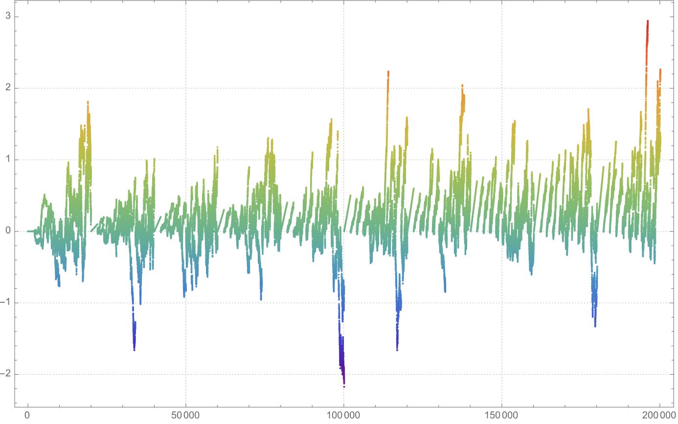
Have you seen the other, the new Brownian Motion Simulator WienerProcess? It's so dynamic it's disgusting. I always wondered how you drew the EEG signal of a cat, a nematode, like that, and how you do the Dynamic content. The color resembles burnt coffee, it's a new world thing. I guess that, I should thank Donavon for being such a pal and for being my ghost philosopher, James for the Brownian Motion Graph, and Varun for the Demonstrations Projects. I asked him and he said...these successor balls just keep coming in and updating, wouldn't it be nice if we could map them all out?
dims = {3, 5};
hallwayThickness = 0.8;
ballCount = 100;
initPs = {1 + hallwayThickness/2, dims[[1]] + hallwayThickness/2};
g = GridGraph[dims];
spanningTree =
FindSpanningTree[GridGraph[dims, EdgeWeight -> {_ :> RandomReal[]}]];
wallsRegion = RegionDifference[
#, Rectangle[{dims[[2]], hallwayThickness},
{dims[[2]], 0} + {hallwayThickness, 1}]] &@
RegionDifference[
Rectangle[{1, 1} - 1 + hallwayThickness, Reverse[dims] + 1],
RegionDilation[
DiscretizeGraphics[
Line[GraphEmbedding[spanningTree][[#]]] & /@
List @@@ EdgeList[spanningTree]],
Rectangle[{0, 0}, {1, 1}*hallwayThickness]]];
positionSeries = Reap[
Sow[ps = ConstantArray[initPs, ballCount]];
While[
And @@ RegionMember[
Rectangle[{1, 1} - 1 + hallwayThickness, Reverse[dims] + 1]][
ps],
vs = RandomPoint[Circle[], ballCount]*0.1; ps += vs;
ps -= vs*Boole[RegionMember[wallsRegion][ps]]; Sow[ps]]][[2,
1]];
winningIndex = FirstPosition[
RegionMember[
Rectangle[{1, 1} - 1 + hallwayThickness, Reverse[dims] + 1]]@
Last@positionSeries, False][[1]];
ballDistanceRanking =
Ordering[
Max /@ Total[(Threaded[initPs] -
Transpose[positionSeries])^2, {3}]]; distanceFromStartGrid =
Function[positions, EuclideanDistance[initPs, #] & /@ positions];
distanceFromEndGrid =
Function[positions,
EuclideanDistance[Reverse[dims] + 1, #] & /@ positions];
plotScatterPlot = Function[{i, distances},
ListPlot[{Transpose[{Range[Length[distances]], distances}],
{{winningIndex, distances[[winningIndex]]}}},
PlotStyle -> {Automatic, Directive[Red, PointSize[Large]],
Directive[Blue, PointSize[Large]]},
PlotTheme -> "Detailed", PlotRange -> All,
ColorFunction -> "Rainbow",
Frame -> True, FrameLabel -> {"i", "Distance Euclidean"},
LabelStyle -> {White, 12}, Background -> White, ImageSize -> 300]];
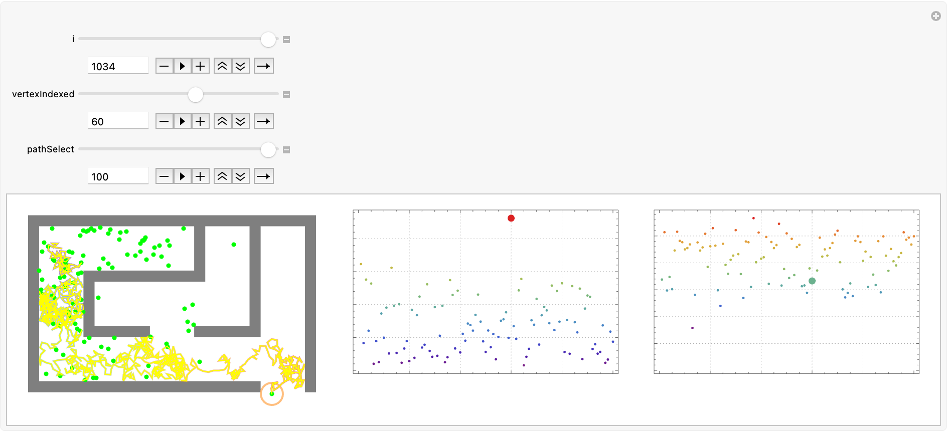
Manipulate[
Row[{Graphics[{Black, Opacity[0.5], wallsRegion,
{Magenta, Thick, Circle[positionSeries[[i, winningIndex]], 0.2],
Thick, Line[positionSeries[[;; i, winningIndex]],
VertexColors -> (ColorData["Rainbow"] /@ Rescale[Range[i]])]},
{Yellow, Thick, Circle[positionSeries[[i, vertexIndexed]], 0.2],
Thin, Line[positionSeries[[All, vertexIndexed]]]},
Green, Opacity[1], PointSize[Medium], Point[positionSeries[[i]]],
Magenta, Opacity[1],
Line[positionSeries[[All, ballDistanceRanking[[pathSelect]]]]],
Yellow, Line[positionSeries[[All, vertexIndexed]]]
}, ImageSize -> 300, Background -> White],
plotScatterPlot[i, distanceFromStartGrid[positionSeries[[i]]]],
plotScatterPlot[i, distanceFromEndGrid[positionSeries[[i]]]]}], {i,
1, Length[positionSeries], 1, Appearance -> "Open",
AnimationRate -> 10},
{vertexIndexed, 1, ballCount, 1, Appearance -> "Open"},
{pathSelect, 1, ballCount, 1, Appearance -> "Open"}]
This is a beautiful topic and I don't know how else to put it. I guess that I really shouldn't have used the resource for vector art, the spanningTree. I did a flip flop, put the old maze back and now we can more clearly delineate the Boolean of wall membership, when you lump it by itself..lump? No, no. Sow the position parts? Sow the position parts. Show how we can get the positionSeries for instance to show the path for one particle field, set some directions for future research. It would be so cool to put some magnetic fields or maybe wind. What would be the meaning of that?
Ya know, how philosophy symbolically reduces to explain the nature of everything. And in this retro simulation we've got a can-full of worms, spider-like paths, in pseudo-random velocity, in a maze. What would you do, if you wanted to in form form the passages and walls and had a FindSpanningTree and GridGraph?
I wonder why maybe because we haven't done experiments on Brownian Motion or not? Because we don't know? Dohh, I don't know. I used to traverse your simulation, last time and actually this is even more fun I think I escaped the big maze and now we've got a new maze. Maze traversal just wouldn't be the same without you.
What is this, a simulation for ants? It's a watercolor made for the ants. That's the extent of, the particles go from the place they're transmitted to the place they're received, which may or may not be the place at which the grid starts and stops.
https://reference.wolfram.com/language/example/BrownianMotion.html
https://demonstrations.wolfram.com/BrownianMotionPathAndMaximumDrawdown/
https://demonstrations.wolfram.com/ExitTimesOfBrownianMotionIn3D/
https://demonstrations.wolfram.com/BrownianMotionIn2DAndTheFokkerPlanckEquation/
https://demonstrations.wolfram.com/TwoDimensionalFractionalBrownianMotion/
And I "tried" to ask some questions about solving mazes outside of the Numberphile video and I couldn't get any kind of a response. I wanted to leverage the random, natural motion of particles to find this maze path and then I would surely simulate the process by which particles might "accidentally" discover an exit. It could be one particle, it could be many particles..but the real question is what comes after and immediately proceeding from the current task at hand which is to follow one particle along a maze-like, core concept. Because when you see the signs and the signals you want to start anthropomorphizing the algorithmic maze-solving methods and when you ask about methods like depth-first search or A* I'm just going to start talking about ants and I did. I provided quite firmly a visual and conceptual link between physical diffusion processes, and computational pathfinding. And I did, I just constructed that maze and let that sit. But it's not enough to just use a spanning tree over a grid. We need the whole thing. We need to make sure we have one unique path between any two points without loops. It may be counterproductive but, it mimics the structure of many real-world mazes. And because the particles travel in a maze, they start from a designated point and move in random directions at each step, reflecting off walls. For now and for the time being we have got to model by collision detection with boundaries so that's set. And then we will be retrieved, essentially, the path of each particle being tracked, but we can model the maximum distance traveled to gather statistical data about the paths to analyze the simulation's..effectiveness..via the path of each particle being tracked. Thus these properties of Brownian motion and random walks become more and more accessible in a visually engaging way, such that allowing users to modify maze configurations or the behavior of particles on the fly could turn the toy simulation into an interactive educational, tool. And that is all.
randomWalk[n_] := Accumulate[
  RandomReal[{-1, 1}, {n, 3}]
  ]
nTurns = 1000;
nParticles = 10;
randomWalks = Table[
   randomWalk[nTurns],
   {i, 1, nParticles}
   ];
crosses = Graphics3D[{
    Red, Sphere[#, 0.3] &
     /@ randomWalks}, Boxed -> False
   ];
lines = ListLinePlot3D[randomWalks,
   Boxed -> False, Axes -> False,
   ColorFunction -> (ColorData["Rainbow"][#3] &),
   ColorFunctionScaling -> False
   ];
Show[lines, crosses]
And I know the moment we start this function it's going to start churning along with this single random walk in three dimensions..cumulatively building up these randomly generated steps where presumably the particles just walk off along the three components representing the z, y, and x directions. But even that semantic component of the step is so much better than when we set the particles on their voyage from the uniform distribution between -1 and 1. And that's the reason why I'm still building this random walk, with fresh new particles in a sequence of 3D positions. We can actually get to this endpoint, and for all this if there's anything that I could have connected it would be creation of these lines over-connecting the steps of all walks. Each walk is represented as a connection of lines in 3D space. The end of each walk, like the Ruliad, is emphasized with a sphere.
nParticles = 10;
nSteps = 1000;
positions = Table[{0.0, 0.0, 0.0}, {nParticles}];
stepSize = 0.5;
steps = RandomReal[{-stepSize, stepSize}, {nSteps, nParticles, 3}];
positions = Accumulate@steps;
animation = Animate[
   ListPointPlot3D[
    Transpose[positions[[1 ;; i, 1 ;; nParticles]]],
    PlotStyle -> Directive[PointSize[0.02], Opacity[0.5]],
    ColorFunction -> Function[{x, y, z}, Hue[(z + 10)/20]],
    ColorFunctionScaling -> False,
    BoxRatios -> {1, 1, 1}, Axes -> False,
    PlotRange -> {{-10, 10}, {-10, 10}, {-10, 10}},
    Lighting -> "Neutral", ImageSize -> Large,
    ViewPoint -> Dynamic[
      RotationMatrix[i*0.01, {0, 0, 1}] . {3, -3, 2}],
    Background -> Transparent],
   {i, 1, nSteps, 1},
   AnimationRepetitions -> 1
   ];
Export["randomWalkAnimation.mp4", animation,
 "VideoEncoding" -> "H264"]
And I know many of us have spent many an evening chatting about how to do a collab between OpenAI and Wolfram on building the Mathematica extension, build an elevated level of abstraction for depicting Brownian Motion, so I took my trusty OpenAI extension and I turned it "into" some prizes that can highlight innovation awards, highlight different possibilities and recognize people who have done some interesting things and so on. Its significance is in highlighting different possibilities and in a sense, providing role models for what's possible and so on. Innovation Awards, I incrementally looked at the path, I looked and saw oh that's why the relevance of what, it's not hard to do what we do. So imagine the simulation of motion of particles influenced by complex wind profiles in a bounded space. The first thing you'll notice is that these particles are stagnant in that they are practically guaranteed to just trail off into the wind but, if we add some rotational motion and simulate wave-like down and up motions along the z-axis then, we get a truly breath-taking weightless computation of the wind influence for each particle's position and what we are applying which is the particle move function that indicates the new position, and we could continue building a second animation block..once we've passed the first animation block then it really is just one illustration of complex particle dynamics in a controlled environment.
nParticles = 10;
nSteps = 200;
stepSize = 0.1;
boxSize = 100.0;
positions = RandomReal[{0, boxSize}, {nParticles, 3}];
vortexInfluence[point_, updraftRate_ : 0.2, maxWindSpeed_ : 0.1] :=
  Module[{x = point[[1]], y = point[[2]], z = point[[3]], r, theta,
    windSpeed}, r = Sqrt[x^2 + y^2];
   theta = ArcTan[x, y];
   windSpeed = Min[r, maxWindSpeed];
   {windSpeed*Cos[theta + Pi/2],
    windSpeed*Sin[theta + Pi/2], (1 - r/boxSize)*updraftRate}];
spiralInfluence[point_, spiralStrength_ : 0.1, growthRate_ : 1] :=
  Module[{x = point[[1]], y = point[[2]], z = point[[3]], r, theta},
   r = Sqrt[x^2 + y^2];
   theta = ArcTan[x, y];
   {spiralStrength*Cos[theta + z/growthRate],
    spiralStrength*Sin[theta + z/growthRate], 0.1}];
sinusoidalInfluence[point_, amplitude_ : 0.1, frequency_ : 0.1] :=
  Module[{x = point[[1]], y = point[[2]], z = point[[3]]}, {0, 0,
    amplitude*Sin[frequency*x]}];
inBoundingBoxQ[point_, boxSize_] :=
 And @@ Thread[Abs[point] <= boxSize/2]
moveParticle[point_, step_, wind_] :=
  With[{newPoint = point + step + wind},
   If[inBoundingBoxQ[newPoint, boxSize], newPoint, point + wind]];
steps = RandomReal[{-stepSize, stepSize}, {nSteps, nParticles, 3}];
positions = Accumulate@steps;
Do[step = steps[[i, j]];
  wind = vortexInfluence[positions[[i, j]]];
  positions[[i + 1, j]] =
   moveParticle[positions[[i, j]], step, wind], {i, nSteps - 1}, {j,
   nParticles}];
animation =
 Animate[ListPointPlot3D[Transpose[positions[[1 ;; i]]],
   PlotStyle -> Directive[PointSize[0.02], Opacity[0.5]],
   ColorFunction -> Function[{x, y, z}, Hue[(z + 10)/20]],
   ColorFunctionScaling -> False, BoxRatios -> {1, 1, 1},
   Axes -> False, PlotRange -> {{-4, 4}, {-4, 4}, {-0, 50}},
   Lighting -> "Neutral", ImageSize -> Large,
   ViewPoint ->
    Dynamic[RotationMatrix[i*0.01, {0, 0, 1}] . {3, -3, 2}],
   Background -> Transparent], {i, 1, nSteps, 1}]
Export["vortexInfluenceAnimation.mp4", animation,
 "VideoEncoding" -> "H264"]
(*positions=Accumulate@steps;
Do[step=steps[[i,j]];
wind=spiralInfluence[positions[[i,j]]];
positions[[i+1,j]]=moveParticle[positions[[i,j]],step,wind],{i,nSteps-\
1},{j,nParticles}];
Animate[ListPointPlot3D[Transpose[positions[[1;;i]]],PlotStyle->\
Directive[PointSize[0.02],Opacity[0.5]],ColorFunction->Function[{x,y,\
z},Hue[(z+10)/20]],ColorFunctionScaling->False,BoxRatios->{1,1,1},\
Axes->False,PlotRange->{{-4,4},{-4,4},{-0,50}},Lighting->"Neutral",\
ImageSize->Large,ViewPoint->Dynamic[RotationMatrix[i*0.01,{0,0,1}].{3,\
-3,2}],Background->Transparent],{i,1,nSteps,1}]
positions=Accumulate@steps;
Do[step=steps[[i,j]];
wind=sinusoidalInfluence[positions[[i,j]]];
positions[[i+1,j]]=moveParticle[positions[[i,j]],step,wind],{i,nSteps-\
1},{j,nParticles}];
Animate[ListPointPlot3D[Transpose[positions[[1;;i]]],PlotStyle->\
Directive[PointSize[0.02],Opacity[0.5]],ColorFunction->Function[{x,y,\
z},Hue[(z+10)/20]],ColorFunctionScaling->False,BoxRatios->{1,1,1},\
Axes->False,PlotRange->{{-1.5,1.5},{-1.5,1.5},{-0,2}},Lighting->"Neutral",\
ImageSize->Large,ViewPoint->Dynamic[RotationMatrix[i*0.01,{0,0,1}].{3,\
-3,2}],Background->Transparent],{i,1,nSteps,1}]*)
So ultimately what ends up happening is the particles, which were merely rolling around in three-dimensional space to begin with, are parameterically apprehended. Specifically, we have to keep changing the parameters (but it's always been that way; no parametric equation starts out with the precise dimensions that we are looking for for any purpose)..and ultimately replace Brownian Motion with parametrically defined and probably a certain typed delineated motion that does for each particle at each step combines the effects of the vortex, spiral, and sinusoidal influences..You name it, Mathematica computes it. The PlotRange quickly adjusts to the interactive, visibility of the particles within the bounding box and, a dynamic view point that clearly adds a rotational effect to the view. And that is how we get this fresh, visual exploration of how the particle physics is what we're doing, we're doing some quick implementation, of a Numberphile video called The Dumbest Way To Solve A Maze in Mathematica. For a quick thought experiment say that you're just standing at a bird's eye view and you say, I want to go see what the particles do in a time series in a unified simulation environment. It's one of these things where the things where, there are people in the biology area who say I'm going to spend my life doing this, the chips don't tend to fall in those directions. It's also something where, it's more of a..something over which the individual doesn't have much control. It's like, unfortunately most of the time with these in retrospect prizes, mostly by the time anybody gets one it's all obvious and irrelevant anyway. It's more interesting these prospective kind of things, here's the thing a prize for promise that could be useful. Back in the days when for example the Nobel Prize was imagined--beginning of the 20th century, there weren't that many people doing basic science. So chances are if something was going to be figured out one or two people et cetera, that was the story. The big experiments and so on have the list of names involved with the experiments, often goes on for more than a page of a journal. It used to be the case, that if there was an article written by 300 people that references to that paper, would say Aardvark et al.. And it's unfortunate for people like me..in modern times the Ws do better because there are transliterations particularly Xs Ys and Zs in Chinese, a recent trend has been since papers are now online ..don't do that just cite everybody! And so you'll see pages that are fifteen pages long! I think it's kind of an interesting situation. I have to say this whole question about AIs doing science and so on, the process of paper production is sort of under attack.
And that's a real sort of value you can get from being in a college environment with real professors. Some people are kind of born project-oriented, but many are not and particularly if you've gone through many years of schooling where it's really about the mechanics of doing things rather than the creating a project and doing it, then it can be one of the main points, a three-week program where kind of one of the big ideas is everyone is going to do an original project. And it's kind of like the mechanics of doing that project, that's a very useful thing for people to learn and I would say a large fraction of people who come to our summer school say they've never done a significant project before this is their first experience with this and, we've been doing our summer school and it's fun to see people who are at the summer school that long ago and by golly they've been continuing doing the projects and being very successful at it. And you can say oh I chipped away at this thing and got started on an assisted project. Many, it depends but I would say that being somewhat modest in the early goals of a project is a good idea. I would say my project is going to be to solve the problem of aging or something and that's your project well, that's a lifetime and more type of project and you won't get that far quickly. But if your project is something much more modest like I'm going something much more incremental, then that's a thing that is much more achievable and you learn a lot; by doing a small project it's not the same for everybody so there are things you will learn about yourself by doing projects. What do I do first with a blank computer screen, a blank sheet of paper and somewhere in the middle you get stuck; work on something different for a while and come back to the thing you were stuck on and your brain may un-stuck itself; actually implement something. There's a small piece that I know how to write Wolfram Language code to do it. And often what I find is not what I expected to find.
And then sort of backing off, looking at something perhaps simpler that I can be concrete about I know I'm not going in the wrong direction building a piece of code is often a way for unsticking things; just try explaining what I'm doing to somebody. I'm sitting and looking at a camera and chatting with you all but, I'm finding a pretty useful mechanism it's even useful to realize that I would have thought I know how this works. Not quite sure but then it kind of crashes and burns as I try to explain it I realize there's a problem here; I have to back off and think about it. Any kind of ego it's just a waste of time I know what to do I don't want to have a big argument about whether we should do this I'm like okay I'm pretty sure this is a good idea let's just do it.
initialFoodSupply = 100;
explorationVolatility = 0.2;
explorationRate = 0.06;
foodDecayRate = 0.03;
explorationDuration = 1;
howMuchExplorations = 1000;
howMuchExplorationSteps = 252;

antFoodSearch[
   currentFood_, explorationIntensity_,
   timeStep_, exploreRate_, decay_, steps_
   ] := Module[
   {
    path = {currentFood},
    rnd,
    stepChange
    },
   Do[
    rnd = RandomVariate[
      NormalDistribution[0, 1]
      ];
    stepChange = (
        exploreRate - decay - 0.5 *explorationIntensity^2
        ) *timeStep + explorationIntensity *Sqrt[timeStep]* rnd;
    AppendTo[
     path,
     Last[path] *Exp[stepChange]
     ],
    {steps}
    ];
   path];

foodFindingStrategy[
   startFood_, intensity_,
   duration_, rate_, decay_,
   threshold_, strategyType_,
   numTrials_, steps_
   ] := Module[
   {paths, finalFoodAmounts, foodGains, effectiveFoodGains},
   paths = Table[
     antFoodSearch[
      startFood, intensity, duration/steps, rate, decay, steps
      ],
     {numTrials}
     ];
   finalFoodAmounts = Last /@ paths;
   foodGains = If[
     strategyType === "explore",
     Max[#, 0] & /@ (finalFoodAmounts - threshold),
     Max[#, 0] & /@ (threshold - finalFoodAmounts)
     ];
   effectiveFoodGains = Exp[-rate*duration]*foodGains;
   {
    Mean[effectiveFoodGains],
    finalFoodAmounts
    }
   ];

{
   exploreGain,
   exploreFoodAmounts
   } = foodFindingStrategy[
   initialFoodSupply,
   explorationVolatility,
   explorationDuration,
   explorationRate,
   foodDecayRate, 100, "explore",
   howMuchExplorations, howMuchExplorationSteps
   ];
{
   abandonGain,
   abandonFoodAmounts
   } = foodFindingStrategy[
   initialFoodSupply,
   explorationVolatility, explorationDuration, explorationRate,
   foodDecayRate, 100, "abandon",
   howMuchExplorations, howMuchExplorationSteps
   ];

samplePaths = Table[
   antFoodSearch[
    initialFoodSupply,
    explorationVolatility,
    explorationDuration/howMuchExplorationSteps, explorationRate,
    foodDecayRate, howMuchExplorationSteps
    ],
   {10}
   ];

ListLinePlot[
 samplePaths,
 PlotRange -> All,
 PlotStyle -> {Thick, Blue},
 Frame -> True,
 FrameLabel -> {"Exploration Step", "Food Amount"},
 PlotLabel -> "Sample Paths of Ant Food Searches",
 PlotTheme -> "Scientific",
 GridLines -> Automatic,
 GridLinesStyle -> Directive[Gray, Dashed],
 PlotLegends -> Placed[
   Automatic,
   Below
   ]
 ]

exploreHistogram = Histogram[
   exploreFoodAmounts,
   {2},
   "ProbabilityDensity",
   Frame -> True,
   FrameLabel -> {"Food Amount", "Probability"},
   PlotLabel ->
    "Distribution of Final Food Amounts for Explore Strategy",
   ChartStyle -> Purple,
   ChartBaseStyle -> EdgeForm[
     White
     ]
   ];

abandonHistogram = Histogram[
   abandonFoodAmounts,
   {2},
   "ProbabilityDensity",
   Frame -> True,
   FrameLabel -> {
     "Food Amount",
     "Probability"
     },
   PlotLabel ->
    "Distribution of Final Food Amounts for Abandon Strategy",
   ChartStyle -> Cyan,
   ChartBaseStyle -> EdgeForm[
     White
     ]
   ];

GraphicsRow[
 {
  exploreHistogram,
  abandonHistogram
  },
 ImageSize -> 800
 ]

Row[
 {
  Style["Explore Strategy Food Gain Estimate: ", Bold, Red],
  exploreGain,
  Spacer[20],
  Style["Abandon Strategy Food Gain Estimate: ", Bold, Blue],
  abandonGain
  }
 ]
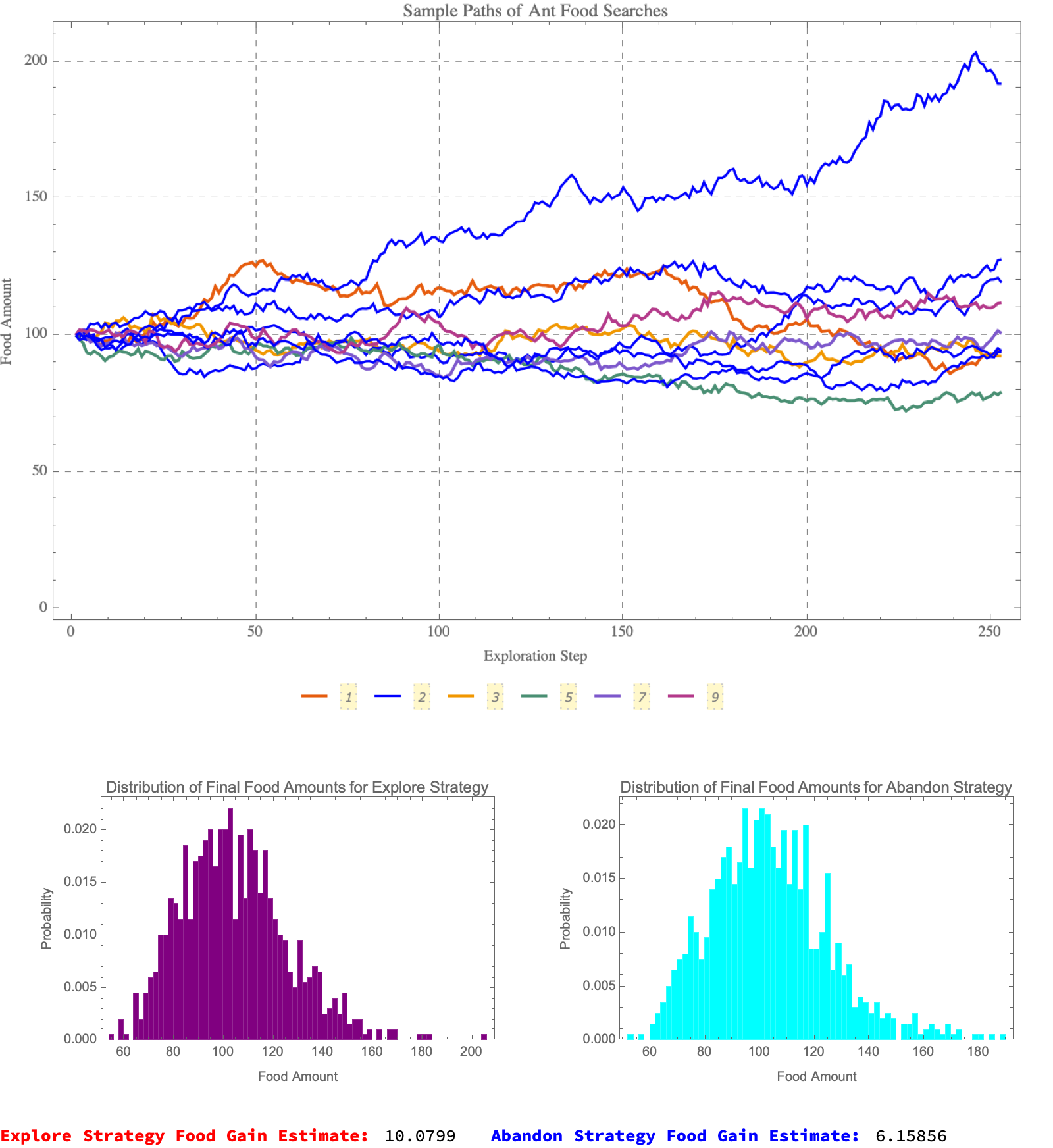
To provide a bit more illumination to yet another corner of the computational universe, out of this Mathematica code we can provide a simulation for an ant colony's food search strategy by modeling the changes in food supply over time based on two different strategies: "explore" and "abandon".. The simulation incorporates stochastic elements to replicate the unpredictability of food availability and environmental conditions. Stemming from the ruins of natural decay or consumption of food over time, we can generate some parameters that hopefully shed some light on concepts like the initial quantity of food available to the ants or, the "volatility" or uncertainty in the food supply change during exploration as well as the rate of exploration with regard to how exploration affects the food supply..as well as the total time spent in exploration. That's not to say that following this strategy or that strategy is intrinsically wrong but that it serves quite semantically as the foundation of the path of food supply change for one trial. In this grid world we can determine the geometry of the Brownian motion model that we determine via the stochastic differential equation withstanding the terms for exploration rate, decay rate, and a random component influenced by the "intensity of exploration". The underlying component of this strategy specification is the multi-way nature of the trials that we run, to simulate different possible outcomes under a specified strategy. And I've calculated all kinds of different strategies and final food amounts and I've adjusted these values, based on the threshold that determines gains from the strategy. The effective gains are in fact discounted by the exploration rate and time to reflect the cost of time in exploration. Identifying pockets of regularity and computational intractability just shows the way that the food finding strategy can be called twice with the preordained strategy parameters that are "explore" and "abandon" to simulate and compare the outcomes of these two strategies. Whereas "exploreGain" and "abandonGain" capture the average gains for each strategy across all trials, which provides an insight into which strategy might be more effective under given conditions. Of course when the 10 trials are over with that's when grid-world ends and we can visualize the sample paths of the food supply, showing how the food supply might evolve over exploration steps under pseudo-random conditions. The following histograms display the distribution of final food amounts for both strategies, giving a visual representation of the variability and expected outcomes of each strategy. I have no idea what they would look like for nested recursive functions. I think writing out the estimated food gains for both strategies provides a quick numerical comparison.
initialFoodSupply = 100;
foodThreshold = 100;
explorationIntensity = 0.2;
explorationRate = 0.06;
foodDecay = 0.03;
explorationDuration = 1;
simCount = 100;
evalCount = 70;
deltaT = explorationDuration/evalCount;
nudt = (explorationRate - foodDecay - (explorationIntensity^2/2))*
deltaT;
normRand := RandomVariate[NormalDistribution[], evalCount];
antMovement[x_] := nudt + explorationIntensity*Sqrt[deltaT]*x;
simulateForaging :=
Module[{paths},
paths = Table[
FoldList[Times, initialFoodSupply,
Exp[antMovement /@ normRand]], {simCount}];
paths];
calculateResourceGain[paths_, strategyType_] := Module[
{finalFoodAmounts, foodGains},
finalFoodAmounts = Last /@ paths;
foodGains = If[
strategyType === "E",
Max[#, 0] & /@ (finalFoodAmounts - foodThreshold),
Max[#, 0] & /@ (foodThreshold - finalFoodAmounts)
];
Mean[
foodGains
]*Exp[
-explorationRate*explorationDuration
]
];
monteCarloStats[gain_] := <|
"Estimate" -> gain,
"StdDev" -> StandardDeviation[Last /@ paths],
"StdError" -> StandardDeviation[Last /@ paths]/Sqrt[simCount]
|>;
paths = simulateForaging;
resourceGainExplore = calculateResourceGain[
paths,
"E"
];
resourceGainAbandon = calculateResourceGain[
paths,
"A"
];
statsExplore = monteCarloStats[
resourceGainExplore
];
statsAbandon = monteCarloStats[
resourceGainAbandon
];
Print[
"Explore Strategy Stats: ",
statsExplore
];
Print[
"Abandon Strategy Stats: ",
statsAbandon
];
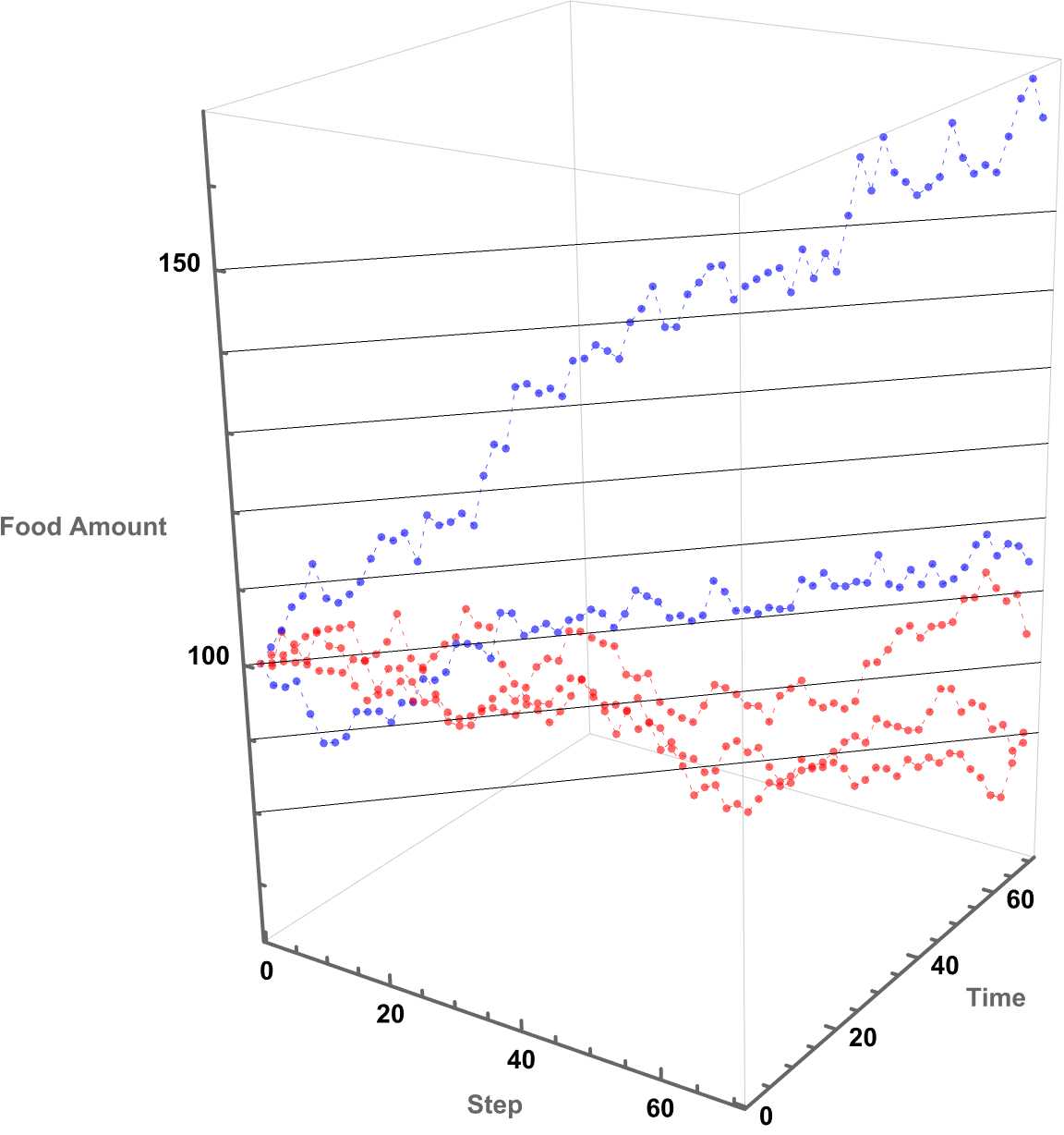
With[{plotStyles =
Table[Directive[Dashing[Small], PointSize[Medium], Opacity[0.6],
If[Last[paths[[i]]] > foodThreshold, Blue, Red]], {i, 1, 5}],
data = Table[
With[{randPath = paths[[i]]},
Table[{j, j, randPath[[j]]}, {j, evalCount}]], {i, 1, 5}],
minFood = Min[Flatten[paths]], maxFood = Max[paths]},
Graphics3D[{Table[{plotStyles[[i]], Line[data[[i]]],
Point[data[[i]]]}, {i, 1, Length[data]}],
FaceGrids -> {{Back, {{0, 1}, {0, 1}}}, {Bottom, {{0, 1}, {0,
1}}}, {Right, {{0, 1}, {0, 1}}}},
FaceGridsStyle -> Directive[Gray, Dashed],
InfiniteLine[{{0, 0, #}, {1, 1, #}}] & /@
Range[Floor[minFood + 20, 10], Ceiling[maxFood - 40, 10], 10]},
Axes -> True, AxesLabel -> {"Step", "Time", "Food Amount"},
PlotRange -> All, Boxed -> True, ImageSize -> Large,
AxesStyle -> Thick, BoxStyle -> Directive[Gray, Thin],
LabelStyle -> {Bold, 14}]]
Manipulate[
Module[
{termFoodAmounts, explorePayoff, abandonPayoff},
termFoodAmounts = paths[[sim]];
explorePayoff = Exp[
-explorationRate*explorationDuration
]*Max[
Last[termFoodAmounts] - foodThreshold,
0
];
abandonPayoff = Exp[
-explorationRate*explorationDuration]*Max[
foodThreshold - Last[termFoodAmounts],
0
];
Column[
{
ListLinePlot[termFoodAmounts,
PlotRange -> {Min[termFoodAmounts]*0.9, Max[termFoodAmounts]*1.1},
GridLines -> Automatic,
AxesLabel -> {"Step", "Food Amount"},
PlotStyle -> If[Last[termFoodAmounts] > foodThreshold, Blue, Red],
PlotTheme -> "Detailed"
],
Text[
Style[
"Explore Payoff: " <> ToString[explorePayoff],
Large
]
],
Text[
Style[
"Abandon Payoff: " <> ToString[abandonPayoff],
Large
]
]
}
]
],
{sim, 1, simCount, 1}
]

frameFunction[simIndex_] :=
  Module[{termFoodAmounts, explorePayoff, abandonPayoff},
   termFoodAmounts = paths[[simIndex]];
   explorePayoff =
    Exp[-explorationRate*explorationDuration]*
     Max[Last[termFoodAmounts] - foodThreshold, 0];
   abandonPayoff =
    Exp[-explorationRate*explorationDuration]*
     Max[foodThreshold - Last[termFoodAmounts], 0];
   ListLinePlot[termFoodAmounts,
    PlotRange -> {Min[termFoodAmounts]*0.9, Max[termFoodAmounts]*1.1},
     GridLines -> Automatic, AxesLabel -> {"Step", "Food Amount"},
    PlotStyle -> If[Last[termFoodAmounts] > foodThreshold, Blue, Red],
     PlotTheme -> "Detailed", Frame -> True,
    FrameLabel -> {"Exploration Step", "Food Amount"},
    PlotLabel ->
     StringJoin["Explore Payoff: ", ToString[explorePayoff], "\n",
      "Abandon Payoff: ", ToString[abandonPayoff]],
    ImageSize -> Large]];
frames = Table[frameFunction[i], {i, 1, simCount}];
Export["foragingSimulation.mp4", frames, "VideoFrames" -> 24];
It's not like you need to know a whole tower, a decade of mathematical knowledge to make progress. By insisting on getting minimal versions of things, you can make progress even without that kind of background educational experience; the more number of people who can get involved in this the better; the better organizational structure probably will call it the Ruliological Society but for now we're launching all these kinds of things at the Wolfram Institute and that's the place where people gathering and hope to build it even further; there's an awful lot to discover and it's like doing any kind of experimental science it's a question of doing clean well organized experiments that you can explain in a clear way. It's sort of inevitable in my experience that sufficiently clear done sufficiently minimal experiments the results are always important. So it's kind of a very encouraging, opportunity for people to do meaningful research that builds up this tower of knowledge that we can make use of in the future. For the time being we have got to preprogram the behavior of the Manipulate object into a set of static frames (which, I've got some bad news--don't have dynamics of their own) which can then be compiled into the following MP4 video.
SeedRandom[1234];
dimensions = {20, 20, 20};
timeSteps = 100;
particles = 50;

noCorrelation = IdentityMatrix[3];
strongCorrelation = {{1, 0.9, 0.9}, {0.9, 1, 0.9}, {0.9, 0.9, 1}};
moderateCorrelation = {{1, 0.5, 0.3}, {0.5, 1, 0.4}, {0.3, 0.4, 1}};

maze = ConstantArray[0, dimensions];

numPipes = 50;
pipeLength = 10;
pipeWidth = 4;

pipePositions = {};
Do[
  direction = RandomChoice[
    {
     {1, 0, 0},
     {0, 1, 0},
     {0, 0, 1}
     }
    ];
  startEdge = RandomChoice[
      {1, dimensions[[#]] - pipeLength + 1}
      ] & /@ Range[3];
  Do[
   Do[
    pos = {
      Clip[
       startEdge[[1]] + i*direction[[1]] + dx,
       {1, dimensions[[1]]}
       ],
      Clip[
       startEdge[[2]] + i*direction[[2]] + dy,
       {1, dimensions[[2]]}
       ],
      Clip[
       startEdge[[3]] + i*direction[[3]] + dz,
       {1, dimensions[[3]]}
       ]
      };
    maze[[Sequence @@ pos]] = 1;
    AppendTo[pipePositions, pos],
    {dx, 0, pipeWidth - 1},
    {dy, 0, pipeWidth - 1},
    {dz, 0, pipeWidth - 1}
    ],
   {i, 0, pipeLength - 1}
   ],
  {numPipes}
  ];

particlePositions = RandomChoice[
   pipePositions,
   particles
   ];

particleColors = Table[
   ColorData["NeonColors", RandomReal[]],
   {particles}
   ];

GenerateCorrelatedBM[dim_, steps_, corrMat_, scale_] := Module[
   {cholDecomp, bm, correlatedSteps},
   cholDecomp = CholeskyDecomposition[corrMat];
   bm = RandomVariate[
     NormalDistribution[0, 1],
     {Length[dim], steps}
     ];
   correlatedSteps = Transpose[
     cholDecomp . bm
     ];
   scale*Accumulate[
     Transpose[
      correlatedSteps
      ]
     ]
   ];

ValidPointQ[pt_, maze_] := AllTrue[
    pt, # > 0 && # <= Dimensions[maze][[1]] &
    ] && maze[[Sequence @@ pt]] == 1;

SolveMazeWithBM[maze_, startPoints_, steps_, corrMat_, scale_] :=
  Module[
   {bmPaths, currentPoints, paths, attempt, maxAttempts = 10,
    nextPoint, valid}, bmPaths = GenerateCorrelatedBM[
     Dimensions[maze], steps, corrMat, scale
     ];
   currentPoints = startPoints;
   paths = Table[
     Reap[
       Do[
        valid = False;
        attempt = 0;
        While[
         ! valid && attempt < maxAttempts,
         nextPoint = Round[currentPoints[[p]] + bmPaths[[All, i]]];
         If[
          ValidPointQ[nextPoint, maze],
          valid = True;
          currentPoints[[p]] = nextPoint;
          Sow[
           nextPoint,
           p
           ],
          bmPaths[[All, i]] = RandomVariate[
            NormalDistribution[0, 1],
            Length[
             Dimensions[maze]
             ]
            ];
          nextPoint = Round[
            currentPoints[[p]] + bmPaths[[All, i]]*scale
            ];
          attempt++]
         ],
        {i, 1, steps}
        ]
       ][[2, 1]],
     {p, 1, Length[startPoints]}
     ];
   paths];

stepSize = 2;
pathsNoCorrelation = SolveMazeWithBM[
   maze, particlePositions, timeSteps, noCorrelation, stepSize
   ];
pathsStrongCorrelation = SolveMazeWithBM[
   maze, particlePositions, timeSteps, strongCorrelation, stepSize
   ];
pathsModerateCorrelation = SolveMazeWithBM[
   maze, particlePositions, timeSteps, moderateCorrelation, stepSize
   ];

Manipulate[
 Graphics3D[
  {
   {Opacity[0.05], LightGreen, EdgeForm[],
    Cuboid /@ Position[maze, 1]},
   Table[
    {
     particleColors[[i]],
     Line[
      Take[paths[[i]], Min[t, Length[paths[[i]]]]]
      ],
     Sphere[
      paths[[i, Min[t, Length[paths[[i]]]]]], 0.2
      ]
     },
    {i, 1, Length[paths]}
    ]
   },
  Axes -> True,
  AxesLabel -> {"X", "Y", "Z"},
  PlotRange -> All,
  Boxed -> False,
  Background -> Transparent
  ],
 {t, 1, timeSteps, 1, ControlType -> Animator, AnimationRate -> 1,
  AnimationRunning -> False},
 {
  {paths, pathsNoCorrelation, "Correlation Type"},
  {pathsNoCorrelation -> "No Correlation",
   pathsModerateCorrelation -> "Moderate Correlation",
   pathsStrongCorrelation -> "Strong Correlation"},
  SetterBar
  }
 ]

frameFunction[paths_, t_] :=
  Graphics3D[{{Opacity[0.05], LightGreen, EdgeForm[],
     Cuboid /@ Position[maze, 1]},
    Table[{particleColors[[i]],
      Line[Take[paths[[i]], Min[t, Length[paths[[i]]]]]],
      Sphere[paths[[i, Min[t, Length[paths[[i]]]]]], 0.2]}, {i, 1,
      Length[paths]}]}, Axes -> True, AxesLabel -> {"X", "Y", "Z"},
   PlotRange -> All, Boxed -> False, Background -> Transparent,
   ImageSize -> Large];
generateFramesForType[paths_] :=
  Table[frameFunction[paths, t], {t, 1, timeSteps}];
framesNoCorrelation = generateFramesForType[pathsNoCorrelation];
framesModerateCorrelation =
  generateFramesForType[pathsModerateCorrelation];
framesStrongCorrelation =
  generateFramesForType[pathsStrongCorrelation];
Export["NoCorrelation.mp4", framesNoCorrelation,
  "VideoEncoding" -> "H264"];(*
Export["ModerateCorrelation.mp4",framesModerateCorrelation,\
"VideoEncoding"->"H264"];
Export["StrongCorrelation.mp4",framesStrongCorrelation,\
"VideoEncoding"->"H264"];
*)
It might seem like it's going to go on Brownian Motion seemingly forever but if we take it further there's a surprise. It seems to kind of resolve itself to something potentially simpler. So what's going on? Let's plot this again but now showing which Colony each Colony is associated with. They start contributing to each other when the correlation is 0.5 and eventually start to exhibit some regularity. And we can kind of home in on the regularity by arranging the Colonies by orthogonal axes and then plotting the axes at each correlation value. We've just got to verify that the path we save it is the working directory. Currently, it's set to "deangladish" firmly. The "VideoFrames" -> 30 option specifies that the video should play at 30 frames per second. And in this correlated foraging motion scenario for three colonies, we use a stochastic model that incorporates correlation between the movements of the colonies instead of simply evaluating a formula. We don't have to follow through all the steps of the computation of the function we can just use this pseudo-formula to work out the result. And it's not worth nothing. And I know this is a bit of a rip but we can set the initial food supplies for the three colonies to the values of 100, 101, and 102 respectively and that allows us to build upon that foundation and represent the intensity or aggressiveness of foraging activities for each colony. Since the food becomes available or regrows at a fixed rate and the food decays or gets consumed naturally without foraging at a fixed rate we can granularly allow the simulation of the correlated foraging motion to sway toward explosive behavior or degenerate behavior depending on the initial environmental or behavioral interactions influencing each other's foraging outcomes. Whichever way the interface swings we can see them the correlation coefficients that don't really categorically affect the foraging paths of the colonies but do provide real-time feedback as we adjust these correlations. It turns out that for any specified initial configuration of values there is only bounded lookback that's the initial value of the function. What we initialize is what we create, that's just the way that we create things. Specifically, we create things in a ..to put it in a different way we have this 3x3 matrix that allows live adjustment of pairwise correlation coefficients among the three colonies, impacting how their food supplies evolve in relation to each other. It's one thing to have independent food supplies for each colony but when the food supply trajectories for each colony over time are all one comparison-visualization of the trends and the interactions that's when we can extend the 2-dimensional line plot to a 3-dimensional point plot that spatially represents all three colonies' food supplies, bringing to life the perception of their interrelated ecological management of resources as well as studies of behavior where understanding the interdependencies and collective behaviors of different groups or species is crucial. But when I put this onto a Mathematica format it's like night and day; we can actually witness whichever way the pendulum swings the theoretical outcomes of different interaction scenarios in a rather controlled environment and if you want something else to sink your teeth into here's the eigen decomposition, the eigensystem of the correlation matrix so that the correlation matrix is positive definite is a thing that adjusts negative eigenvalues to be slightly positive (0.01 offset) and thus the matrix is positive definite, suitable for Cholesky decomposition of the adjusted correlation matrix to facilitate the generation of correlated random steps.
initialFoodSupply = {100, 101, 102};
foragingIntensity = {0.2, 0.25, 0.3};
foodGrowthRate = 0.06;
foodDecayRate = 0.03;
foragingDuration = 1;
evaluationSteps = 100;

correlatedForagingMotion[
   initialFood_, intensities_, growthRate_, decayRate_, duration_,
   steps_, correlations_
   ] := Module[
   {
    L, dt, foodIncreases, foodIntakes, paths, initialLogFood,
    valid, eigenSys, eigenValues, eigenVectors, nearestPD
    },
   eigenSys = Eigensystem[correlations];
   eigenValues = eigenSys[[1]];
   eigenVectors = eigenSys[[2]];
   nearestPD = eigenVectors . DiagonalMatrix[
      0.01 + Max[
          0, #] & /@ eigenValues] . Transpose[
      eigenVectors];
   L = CholeskyDecomposition[
     nearestPD];
   dt = duration/steps;
   foodIncreases = (
      growthRate - decayRate - intensities^2/2)  dt;
   foodIntakes = (
      intensities Sqrt[dt])  L;
   initialLogFood = Log[
     initialFood];
   paths = Table[
     initialLogFood, {steps}];
   Do[
    paths[[i + 1]] =
     paths[[i]] + foodIncreases + foodIntakes . RandomVariate[
        NormalDistribution[0, 1],
        Length[initialFood]
        ],
    {i, 1, steps - 1}
    ];
   Exp[paths]];

Manipulate[
 correlatedPaths = correlatedForagingMotion[
   initialFoodSupply, foragingIntensity, foodGrowthRate,
   foodDecayRate, foragingDuration, evaluationSteps,
   {
    {1, corr12, corr13},
    {corr12, 1, corr23},
    {corr13, corr23, 1}
    }
   ];
 plotCorrelatedForagingPaths = ListLinePlot[
   Transpose[correlatedPaths],
   PlotRange -> All,
   AxesLabel -> {"Time", "Food Supply"},
   PlotLegends -> {"Colony 1", "Colony 2", "Colony 3"},
   PlotLabel -> "Correlated Foraging Paths",
   Joined -> True,
   ImageSize -> Medium
   ];
 plotCorrelatedForagingPaths3D = ListPointPlot3D[
   Transpose[
    Table[
     correlatedPaths[[All, i]],
     {i, 1, 3}
     ]
    ],
   PlotRange -> All,
   AxesLabel -> {"Colony 1", "Colony 2", "Colony 3"},
   PlotLegends -> Placed["Each Colony is Associated With", Below],
   PlotStyle -> PointSize[Small],
   PlotLabel -> "Correlated Foraging in 3D",
   ImageSize -> Medium
   ];
 Column[
  {
   plotCorrelatedForagingPaths,
   plotCorrelatedForagingPaths3D
   }
  ],
 {
  {corr12, 0.5, "Correlation 1-2"},
  -1, 1, 0.1,
  Appearance -> "Labeled"
  },
 {
  {corr13, 0.2, "Correlation 1-3"},
  -1, 1, 0.1,
  Appearance -> "Labeled"
  },
 {
  {corr23, -0.4, "Correlation 2-3"},
  -1, 1, 0.1,
  Appearance -> "Labeled"
  },
 TrackedSymbols :> {
   corr12, corr13, corr23
   }
 ]
Functions that were defined recursively were the hardest to guess; Douglas Hofstadter, he sent a letter to Neil Sloane in what's now the encyclopedia of integer sequences or OEIS. These sequences have a very regular form that we would call nested. But actually as we saw above a small change in initial conditions would have led to much wilder behavior but that wasn't something Doug happened to notice. There was another nestedly recursive sequence that Doug described as a force of an entirely another color; he quotes, absolutely CRAZY, Q-Sequence. In it, tucked away at the bottom of page 137, a few pages after discussion of strange bagels that the purple cow without horns gobbled..Doug's "Eta-sequences"...but as Doug pointed out, the nested form properties Douglas seemed most concerned about in the letter. And this was shoved down my throat in the context of the exemplification of the "butterfly effect" within chaotic systems. In the context of recursive sequences, such sensitivities can make the long-term prediction of sequence values highly unpredictable, even if the generating rules are simple and deterministic.
corr12Values = Range[-1, 1, 0.2];
corr13Values = Range[-1, 1, 0.2];
corr23Values = Range[-1, 1, 0.2];
generateFrames[corr12_, corr13_, corr23_] :=
  Module[{correlatedPaths, plot2D, plot3D},
   correlatedPaths =
    correlatedForagingMotion[initialFoodSupply, foragingIntensity,
     foodGrowthRate, foodDecayRate, foragingDuration,
     evaluationSteps, {{1, corr12, corr13}, {corr12, 1,
       corr23}, {corr13, corr23, 1}}];
   plot2D =
    ListLinePlot[Transpose[correlatedPaths], PlotRange -> All,
     AxesLabel -> {"Time", "Food Supply"},
     PlotLegends -> {"Colony 1", "Colony 2", "Colony 3"},
     Joined -> True, ImageSize -> Large];
   plot3D =
    ListPointPlot3D[
     Transpose[Table[correlatedPaths[[All, i]], {i, 1, 3}]],
     PlotRange -> All,
     AxesLabel -> {"Colony 1", "Colony 2", "Colony 3"},
     PlotLegends -> Placed["Each Colony is Associated With", Below],
     PlotStyle -> PointSize[Medium], ImageSize -> Large];
   {plot2D, plot3D}];
frames =
  Flatten[Table[
    generateFrames[corr12, corr13, corr23], {corr12,
     corr12Values}, {corr13, corr13Values}, {corr23, corr23Values}],
   2];
Export["CorrelatedForagingAnimation.mp4", frames,
  "VideoFrames" -> 30];
And so given these initial resources as well as parameters for volatility, growth, and decay, we can accumulate resources via the geometric Brownian motion model where each step's change is determined by both deterministic (growth and decay) and stochastic (volatility) factors. That means that the two types of payoffs that are calculated - explore payoff and abandon payoff - can be representative of the strategies of continuing to explore (accumulate and generate resources beyond a threshold) or abandon (resources dropping below the boundary threshold) respectively. The payoffs are discounted by the growth rate over the period to account for time value. That's why we need to decompose and define the correlation matrix using the Cholesky decomposition..this allows the creation of correlated random variates needed for the simulation. By looking at the way that multiple resource pools can be measured across correlation, we can potentially simulate resource levels across different pools using the derived factors from the Cholesky decomposition, which is how interaction is attached to the pools through the correlation structure. That is how the differentiation of the simulations proceeds; the users can dynamically select different simulation runs and observe the correlated real-time display not just of the behaviors of the resource pools but of their attributes as defined by the hard-coded volatility, growth, decay, and mutual correlations as well as the correlation matrices and geometric Brownian motion under stochastic conditions. That's why knitting together all those threads of interactions is being explicitly realized in the sense of how the interactive exploration of the simulation outcomes takes place.
We're really saying there's an underlying structure to do with these things like branchial graphs, multiway graphs, that is the way that the universe is actually built and that gives you this object that leads to quantum mechanics. There's vastly more to figure out about how that thing works, now there's all sorts of effects that that thing suggests you know that the physical space at the speed of light there's this space of possible quantum histories, possible quantum branches that we call the maximum entanglement speed and that sort of limits the rate of propagation in branchial space and I suspect that quantity is related to the limitations on quantum measurement processes and that thing is a direction to go in. What's happening in quantum mechanics is that one electrons, two electrons, three electrons..it's become quite good when those things are not coupled pretty strongly, one can work out what happens with small numbers of particles. By the time you're dealing with large numbers of particles, that's when that's important..a size that we can actually sense, it's extremely difficult to come up with a formalism that can describe what's going on except in special cases. The propagation of electrons in solids in crystals, there's a regular background lattice in which electrons move and that regularity is sort of intractable in terms of quantum mechanics and what's going on. And I think that's sort of a frontier problem that affects the progress that's been made--superfluid liquid helium, is a sort of fundamentally quantum phenomenon. Superfluids have a feature that everything moves together; one can somewhat reduce the accounting for many different particles to something a bit simpler in that case. And I don't know for sure but I have a suspicion that this approach that we have taken could be a good way to approach that; we can only do a certain amount of computation, and the universe when it figures out what happened in a quantum situation is an aspect of what the universe does; we can do a cheap computation and jump ahead and see what happens. What kinds of cheap computations are possible is not clear.
ClearAll["Global`*"];
SeedRandom[123];
initialResources = 100;
resourceThreshold = 100;
resourceVolatility = 0.2;
environmentalGrowthRate = 0.06;
resourceDecayRate = 0.03;
foragingPeriod = 1;
simulations = 500;
evaluationSteps = 63;
dt = foragingPeriod/evaluationSteps;
simulateResourceAccumulation[
initial_, vol_, growthRate_, decay_, threshold_, steps_, sims_
] := Module[
{paths, explorePayoff, abandonPayoff}, paths = Table[
FoldList[
#1*Exp[
(growthRate - decay - 0.5*vol^2)*dt +
vol*Sqrt[dt]*RandomVariate[NormalDistribution[]]] &,
initial,
Array[Null &, steps - 1]
],
{sims}
];
explorePayoff = Exp[
-growthRate*foragingPeriod
]*Max[
Last[#] - threshold, 0
] & /@ paths;
abandonPayoff = Exp[
-growthRate*foragingPeriod
]*Max[
threshold - Last[#],
0
] & /@ paths;
<|
"Explore Foraging Value" -> Mean[explorePayoff],
"Abandon Foraging Value" -> Mean[abandonPayoff],
"Explore Std Dev" -> StandardDeviation[explorePayoff],
"Abandon Std Dev" -> StandardDeviation[abandonPayoff]
|>
];
result = simulateResourceAccumulation[
initialResources, resourceVolatility, environmentalGrowthRate,
resourceDecayRate, resourceThreshold, evaluationSteps, simulations
];
result // Dataset
correlationMatrix = {
{1, 0.5, 0.2},
{0.5, 1, -0.4},
{0.2, -0.4, 1}
};
choleskyDecomp = CholeskyDecomposition[
correlationMatrix];
initialResourceLevels = {
100, 101, 98};
growthRates = {
0.03, 0.06, 0.02};
volatilityRates = {
0.05, 0.2, 0.15};
simulateCorrelatedExploration[
resources_, growthRates_, volatilities_,
chol_, steps_, sims_] := Module[
{paths}, paths = Table[
FoldList[
#1*
Exp[(growthRates - 0.5*volatilities^2)*dt +
chol . volatilities*Sqrt[dt]*#2] &,
resources,
RandomVariate[
NormalDistribution[0, 1],
{steps, 3}
]
],
{sims}
];
paths];
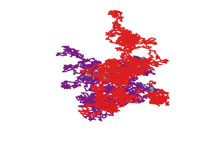
correlatedPaths = simulateCorrelatedExploration[
initialResourceLevels, growthRates, volatilityRates,
choleskyDecomp, evaluationSteps, simulations
];
purpleShades = Table[
Blend[
{RGBColor[0.4, 0.2, 0.8], Magenta},
i/(Length[correlatedPaths] - 1)
],
{i, 0, Length[correlatedPaths] - 1}
];
Manipulate[
ListLinePlot3D[
correlatedPaths[[simulationIndex]],
AxesLabel -> {"Resource Pool 1", "Resource Pool 2",
"Resource Pool 3"},
PlotLabel ->
"3D Correlated Resource Levels for Three Resource Pools",
PlotRange -> All,
BoxRatios -> {1, 1, 1},
PlotStyle -> Directive[
purpleShades[[simulationIndex]],
Thick
],
Mesh -> All,
MeshStyle -> Directive[
PointSize[Large],
purpleShades[[simulationIndex]]
]
],
{
{
simulationIndex, 1, "Simulation Index"
},
1,
Length[correlatedPaths],
1
}
]
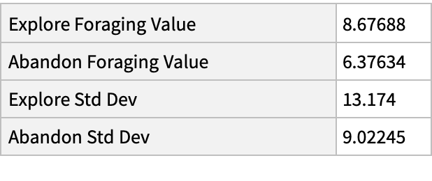
I always thought that the sign of gene editing happening is when you get glow in the dark humans and you get a fashion statement for having your skin glow in the dark. Jellyfish, fish and the jellyfish gene inserted into them..there is supposedly a plant that glows in the dark I've ordered one it hasn't come yet there is supposedly a plant that glows in the dark because it has jellyfish genes in it; there are aspects of glowing in the dark when one's trying to insert this series of computations and visualizations designed to model the accumulation of resources in an environment with defined growth, decay rates, and volatilities under a correlated setting among multiple resource pools and produce light when we do things like graph these parameters including the initial resources as well as the thresholds for those resources..we can plot the volatility as well as the rates at which the accumulation of resources grows and decays via the number of simulations and the steps that it takes to evaluate the process of resource accumulation over time. As usual we use the geometric Brownian motion "GBM" model which is a big mess because we have got to iteratively calculate the resource levels at each step using an exponential growth factor influenced, by the specified rates and thus we get this dataset that makes changes to the explore foraging value (that is the average payoff when continuing to exploit resources beyond a certain threshold) and the abandon foraging value (that is the average payoff when ceasing all exploitation of resources below a certain threshold).
frameFunction[index_] :=
  ListLinePlot3D[correlatedPaths[[index]],
   AxesLabel -> {"Resource Pool 1", "Resource Pool 2",
     "Resource Pool 3"},
   PlotLabel ->
    "3D Correlated Resource Levels for Three Resource Pools",
   PlotRange -> All, BoxRatios -> {1, 1, 1},
   PlotStyle -> Directive[purpleShades[[index]], Thick], Mesh -> All,
   MeshStyle -> Directive[PointSize[Large], purpleShades[[index]]]];
frames = Table[frameFunction[i], {i, 1, Length[correlatedPaths]}];
Export["CorrelatedResourceExploration.mp4", frames,
  "VideoEncoding" -> "H264"];
Now, when you have multiple resource pools with correlated changes, you can simulate the paths for each resource pool, taking into account the specific growth rates and volatilities, the correlations derived from the Cholesky decomposition. The most important thing is to plan your interaction via this absolutely bewitched gradient it's all purple and shades, of purple which provides the visual distinction between the different simulations. We can cycle through different simulation runs and as we run the simulation we can observe how these resources evolve over time under the correlated dynamics with labelled axes for each and every resource pool and, the generative purple shades are what give us the visual en-coding of different simulation runs it's like running a spaghetti code kind of marathon mess of how stochastic modeling works. At least for a while, the phenomenon of computational irreducibility--just because you know the rules for a system doesn't mean you know how it's going to behave..I really want my kid to have green eyes. I really want to offer insights into the complex interactions between multiple resource pools in a correlated environment.
currentResources = 100;
desiredThreshold = 100;
resourceVolatility = 0.2;
environmentalGrowthRate = 0.06;
resourceDecayRate = 0.03;
foragingDuration = 1;
foragingSimulations = 500;
foragingSteps = 63;
dt = foragingDuration/foragingSteps;
simulateForaging[current_, vol_, growth_, decay_, threshold_, steps_,
   sims_] :=
  Module[{paths, successGather, failGather},
   paths = Table[
     FoldList[#1*
        Exp[(growth - decay - 0.5*vol^2)*dt +
          vol*Sqrt[dt]*RandomVariate[NormalDistribution[]]] &,
      current, Array[Null &, steps - 1]], {sims}];
   successGather =
    Exp[-growth*foragingDuration]*Max[Last[#] - threshold, 0] & /@
     paths;
   failGather =
    Exp[-growth*foragingDuration]*Max[threshold - Last[#], 0] & /@
     paths;
   <|"Successful Foraging Mean" -> Mean[successGather],
    "Failed Foraging Mean" -> Mean[failGather],
    "Successful Foraging Std Dev" -> StandardDeviation[successGather],
     "Failed Foraging Std Dev" -> StandardDeviation[failGather]|>];

Manipulate[
 Module[{resources, paths, finalPaths, meanPaths, choleskyDecomp, dt,
   colors, meanPlot, pointPlot, foragingResults, successMean,
   failMean, successStdDev, failStdDev, covarianceMatrix},
  dt = foragingDuration/foragingSteps;
  choleskyDecomp = CholeskyDecomposition[correlationMatrix];
  resources = initialResources;
  colors =
   Table[ColorData["Rainbow"][(i - 1)/(foragingSimulations - 1)], {i,
     foragingSimulations}];
  paths =
   Table[FoldList[#1*
       Exp[(muVec - 0.5 sigmaVec^2)*dt +
         choleskyDecomp . sigmaVec*Sqrt[dt]*#2] &, resources,
     RandomVariate[
      NormalDistribution[0, 1], {foragingSteps,
       3}]], {foragingSimulations}];
  finalPaths = Transpose[paths, {3, 2, 1}];
  meanPaths = Mean /@ Transpose[paths, {3, 2, 1}];
  foragingResults =
   simulateForaging[resources[[1]], sigmaVec[[1]],
    environmentalGrowthRate, resourceDecayRate, desiredThreshold,
    foragingSteps, foragingSimulations];
  successMean = foragingResults["Successful Foraging Mean"];
  failMean = foragingResults["Failed Foraging Mean"];
  successStdDev = foragingResults["Successful Foraging Std Dev"];
  failStdDev = foragingResults["Failed Foraging Std Dev"];
  covarianceMatrix =
   correlationMatrix*Outer[Times, sigmaVec, sigmaVec];
  pointPlot =
   ListPointPlot3D[finalPaths, PlotRange -> All,
    AxesLabel -> Style[#, Larger, Bold] & /@ {"Resource Pool 1",
      "Resource Pool 2", "Resource Pool 3"},
    PlotLabel -> Style["3D Correlated Resource Levels", Bold, Larger],
     BoxRatios -> {1, 1, 1}, ImageSize -> 300,
    PlotStyle -> Thread[PointSize[Medium]*colors],
    Background -> Transparent, AxesStyle -> Directive[Black, Thick]];
  meanPlot =
   ListPlot[meanPaths, Joined -> True,
    PlotLegends -> {"Resource Pool 1", "Resource Pool 2",
      "Resource Pool 3"},
    PlotLabel ->
     Style["Mean Path of Resource Accumulation", Bold, Larger],
    AxesLabel -> {"Time", "Resources"}, ImageSize -> 200,
    ImagePadding -> {{40, 40}, {40, 40}}];
  Column[{pointPlot, meanPlot,
    Style[Grid[{{"Successful Foraging Mean:",
        successMean}, {"Failed Foraging Mean:",
        failMean}, {"Successful Standard Deviation:",
        successStdDev}, {"Failed Standard Deviation:",
        failStdDev}, {"Covariance Matrix:",
        MatrixForm[covarianceMatrix]}}], Bold,
     Larger]}]], {{correlationMatrix, {{1, 0.5, 0.2}, {0.5,
     1, -0.4}, {0.2, -0.4, 1}}, "Correlation Matrix"},
  ControlType -> InputField,
  FieldSize -> {32, 3}}, {{initialResources, {100, 101, 98},
   "Initial Resources"}, ControlType -> InputField,
  FieldSize -> {10, 3}}, {{muVec, {0.03, 0.06, 0.02}, "Growth Rates"},
   ControlType -> InputField,
  FieldSize -> {10, 3}}, {{sigmaVec, {0.05, 0.2, 0.15},
   "Resource Volatilities"}, ControlType -> InputField,
  FieldSize -> {10, 3}}, {environmentalGrowthRate, 0.06,
  "Environmental Growth Rate", 0.01, 0.1, 0.01}, {resourceDecayRate,
  0.03, "Resource Decay Rate", 0.0, 0.1, 0.01}, {desiredThreshold,
  100, "Desired Threshold", 80, 120, 1}, {foragingDuration, 1,
  "Foraging Duration", 0.1, 2, 0.1}, {foragingSteps, 252,
  "Foraging Steps", 100, 500, 1}, {foragingSimulations, 50,
  "Foraging Simulations", 10, 100, 1},
 TrackedSymbols -> {correlationMatrix, initialResources, muVec,
   sigmaVec, environmentalGrowthRate, resourceDecayRate,
   desiredThreshold, foragingDuration, foragingSteps,
   foragingSimulations}]
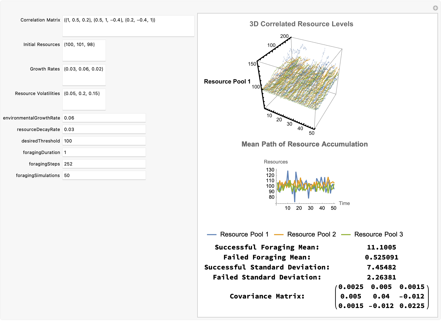
It might be helpful to think of the explore payoff..as the gain from resources that exceed the threshold after the foraging period, adjusted by the exponential of the negative growth rate over the duration, representing the opportunity cost or risk of waiting. We don't want to do something that would make us feel bad. We don't want to impose that on other things that are like us enough that we can kind of infer that they would feel pain as we feel pain so to speak and that's obviously an issue, with the abandon payoff wherein we retrieve some loss (or avoided cost) from the resources that fall below the threshold! That is how we return the statistical version of the mean and standard deviation which might provide some insight into the expected outcomes of foraging strategies under uncertainty. That is how the mean paths plot works because we're averaging the paths across simulations for the expected resource accumulation over time, to gain a fresh perspective and most of all to present these ..not with too much self referential reflection but we should state that the simulation does respect the intended relationships between different resource pools.
ClearAll["Global`*"]
dims2D = {10, 10};
maze2D = ConstantArray[1, dims2D];

walls2D = {{1, 2}, {1, 5}, {2, 2}, {3, 3}, {3, 7}, {4, 5}, {5, 8}, {6,
     1}, {7, 7}, {8, 4}, {9, 9}};
Do[maze2D[[wall[[1]], wall[[2]]]] = 0, {wall, walls2D}];

mu2D = {0, 0};
sigma2D = {{0.1, 0.05}, {0.05, 0.1}};
steps2D = 500;

startPoint2D = {1, 1};
endPoint2D = {10, 10};

paths2D =
  Table[Module[{path = {startPoint2D}, point = startPoint2D, i = 1},
    While[i <= steps2D && point != endPoint2D,
     point = path[[-1]] +
       RandomVariate[MultinormalDistribution[mu2D, sigma2D]];
     point = Round[point];
     If[1 <= point[[1]] <= dims2D[[1]] &&
       1 <= point[[2]] <= dims2D[[2]] &&
       maze2D[[point[[1]], point[[2]]]] == 1, AppendTo[path, point];
      i++;];];
    path], {10}];

dims3D = {10, 10, 10};
maze3D = ConstantArray[1, dims3D];

walls3D = {{1, 2, 3}, {2, 5, 6}, {3, 7, 4}, {4, 5, 5}, {5, 8, 3}, {6,
    1, 7}, {7, 7, 8}, {8, 4, 2}, {9, 9, 9}, {10, 5, 1}};
Do[maze3D[[wall[[1]], wall[[2]], wall[[3]]]] = 0, {wall, walls3D}];

mu3D = {0, 0, 0};
sigma3D = {{0.1, 0.05, 0.03}, {0.05, 0.1, 0.02}, {0.03, 0.02, 0.1}};
steps3D = 1000;

startPoint3D = {1, 1, 1};
endPoint3D = {10, 10, 10};

paths3D =
  Table[Module[{path = {startPoint3D}, point = startPoint3D, i = 1},
    While[i <= steps3D && point != endPoint3D,
     point = path[[-1]] +
       RandomVariate[MultinormalDistribution[mu3D, sigma3D]];
     point = Round[point];
     If[1 <= point[[1]] <= dims3D[[1]] &&
       1 <= point[[2]] <= dims3D[[2]] &&
       1 <= point[[3]] <= dims3D[[3]] &&
       maze3D[[point[[1]], point[[2]], point[[3]]]] == 1,
      AppendTo[path, point];
      i++;];];
    path], {10}];

Graphics[{{LightGray,
   Table[If[maze2D[[i, j]] == 0, {Black, Rectangle[{i, j}]},
     Nothing], {i, dims2D[[1]]}, {j, dims2D[[2]]}]}, {Table[
    If[Last[paths2D[[i]]] == endPoint2D, {Green,
      Line[paths2D[[i]]]}, {Red, Line[paths2D[[i]]]}], {i,
     Length[paths2D]}]}, {Green, Disk[startPoint2D, 0.2]}, {Blue,
   Disk[endPoint2D, 0.2]}}, Frame -> True, FrameTicks -> None,
 GridLines -> Automatic]

Graphics3D[{{LightGray,
   Table[If[maze3D[[i, j, k]] == 0, {Black, Cuboid[{i, j, k}]},
     Nothing], {i, dims3D[[1]]}, {j, dims3D[[2]]}, {k,
     dims3D[[3]]}]}, {Table[
    If[Last[paths3D[[i]]] == endPoint3D, {Green,
      Line[paths3D[[i]]]}, {Red, Line[paths3D[[i]]]}], {i,
     Length[paths3D]}]}, {Green, Sphere[startPoint3D, 0.3]}, {Blue,
   Sphere[endPoint3D, 0.3]}}, Boxed -> True, Axes -> True,
 AxesLabel -> {"X", "Y", "Z"}]
But it seems that the pathfinding in two-dimensional and three-dimensional "2D" and "3D" shapes in these mazes, one can sort of hack biology and kind of find these weak links and it becomes a problem much like computer security. In the sense that we can experimentally use a random walk modeled by a multivariate normal distribution, influenced by specified mean vectors and covariance matrices..this is the simulation step that we use and we use it quite frequently it's actually quite typical for our computational modeling approach, to understand stochastic processes. Pick an animal like an ant and you will see them in the Ruliad, how the Ruliad permeates through everything I was watching an ant in some confined spaces. I was ready to observe some molecular motion throughout two-dimensional grid mazes and place walls and block movement and all that jazz but I didn't know how I was too new to learning how to build a maze and generate multiple paths through that maze 2D or even 3D using a random walk..but then I saw the Mathematica icon and I knew the meaning of generating multiple paths, through the two-dimensional maze and in fact we were able to continue until the endpoint was reached or the maximum number of steps reached exhaustion.
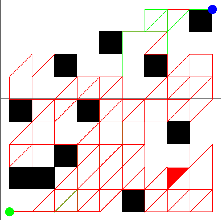
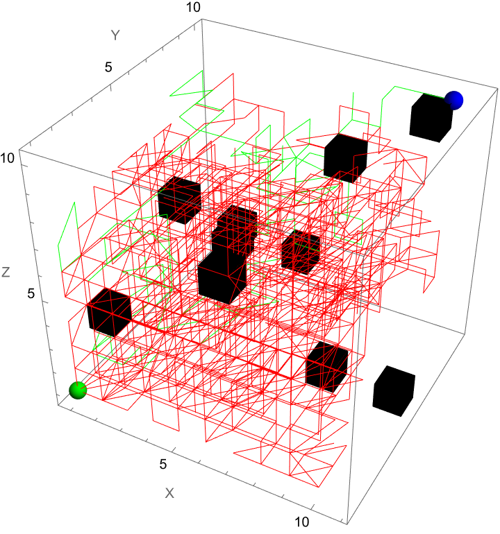
Biological evolution is sort of a way of finding solutions to things. Finding that way of having to manage the bacterium and Mathematica knows how to do that! None of that would matter unless we can actually do that so we can mark the beginning and end of the maze and then generate some paths, it was getting 10 to the fortieth different tries of different things which succeed or fail about a trillion generations of organisms have lived. That's a sense of scale of what you get to try there. A similar approach is what we take in 3D, in that we have these paths that are rendered as lines through a cube and of that we can successfully and or unsuccessfully color-code these paths which we can potentially do in constrained environments like mazes. So whether it's robotics --for pathfinding in uncertain environments--or ecology--to understand animal movement patterns within habitats--or even finance--to model the random behavior of stock prices within defined ranges--it's a question of if the movement tendencies have been properly formatted and respectfully specified via the use of covariance matrices, which allow us to correlate movements in dimensions that are different. And in this corner of the Ruliad we tend to suggest that left to their own devices, the wind and water currents in environmental studies they know, that they are inter-dependent.
dims2D = {10, 10};
startPoint2D = {1, 1};
endPoint2D = {10, 10};
mu2D = {0, 0};
sigma2D = {{0.1, 0.05}, {0.05, 0.1}};
steps2D = 1000;
walls2D = {{1, 2}, {1, 5}, {2, 2}, {3, 3}, {3, 7}, {4, 5}, {5, 8}, {6,
     1}, {7, 7}, {8, 4}, {9, 9}};
maze2D = ConstantArray[1, dims2D];
Do[maze2D[[wall[[1]], wall[[2]]]] = 0, {wall, walls2D}];

dims3D = {10, 10, 10};
startPoint3D = {1, 1, 1};
endPoint3D = {10, 10, 10};
mu3D = {0, 0, 0};
sigma3D = {{0.1, 0.05, 0.03}, {0.05, 0.1, 0.02}, {0.03, 0.02, 0.1}};
steps3D = 2000;
walls3D = {{1, 2, 3}, {2, 5, 6}, {3, 7, 4}, {4, 5, 5}, {5, 8, 3}, {6,
    1, 7}, {7, 7, 8}, {8, 4, 2}, {9, 9, 9}, {10, 5, 1}};
maze3D = ConstantArray[1, dims3D];
Do[maze3D[[wall[[1]], wall[[2]], wall[[3]]]] = 0, {wall, walls3D}];

simulate2DPath[_][_][0] = startPoint2D;
simulate2DPath[mu_][sigma_][steps_] :=
  simulate2DPath[mu][sigma][steps] =
   Module[{},
    point = simulate2DPath[mu][sigma][steps - 1] +
      RandomVariate[MultinormalDistribution[mu, sigma]];
    point = Round[point];
    If[1 <= point[[1]] <= dims2D[[1]] &&
      1 <= point[[2]] <= dims2D[[2]] &&
      maze2D[[point[[1]], point[[2]]]] == 1, point,
     simulate2DPath[mu][sigma][steps]]];

simulate3DPath[_][_][0] = startPoint3D;
simulate3DPath[mu_][sigma_][steps_] :=
  simulate3DPath[mu][sigma][steps] =
   Module[{},
    point = simulate3DPath[mu][sigma][steps - 1] +
      RandomVariate[MultinormalDistribution[mu, sigma]];
    point = Round[point];
    If[1 <= point[[1]] <= dims3D[[1]] &&
      1 <= point[[2]] <= dims3D[[2]] &&
      1 <= point[[3]] <= dims3D[[3]] &&
      maze3D[[point[[1]], point[[2]], point[[3]]]] == 1, point,
     simulate3DPath[mu][sigma][steps]]];

simulate2DAnimationPath[mu_][sigma_][steps_] :=
  Module[{reached = False, prepost = {}},
   ListAnimate[
    Table[prepost =
      TakeWhile[
       Table[simulate2DPath[mu][sigma][i], {i, 0, step}], # !=
         endPoint2D &];
     Graphics[{LightGray,
       Table[If[maze2D[[i, j]] == 0, {Black, Rectangle[{i, j}]},
         Nothing], {i, dims2D[[1]]}, {j, dims2D[[2]]}], Green, Thick,
       Line[prepost], Orange,
       Line[Table[
         simulate2DPath[mu][sigma][i], {i, Length[prepost] + 1,
          step}]], Green, Disk[startPoint2D, 0.2], Blue,
       Disk[endPoint2D, 0.2]}, Frame -> True, FrameTicks -> None,
      GridLines -> Automatic], {step, 0, steps, 10}]]];

simulate3DAnimationPath[mu_][sigma_][steps_] :=
  Module[{reached = False, prepost = {}},
   ListAnimate[
    Table[prepost =
      TakeWhile[
       Table[simulate3DPath[mu][sigma][i], {i, 0, step}], # !=
         endPoint3D &];
     Graphics3D[{LightGray,
       Table[If[maze3D[[i, j, k]] == 0, {Black, Cuboid[{i, j, k}]},
         Nothing], {i, dims3D[[1]]}, {j, dims3D[[2]]}, {k,
         dims3D[[3]]}], Green, Thick, Line[prepost], Orange,
       Line[Table[
         simulate3DPath[mu][sigma][i], {i, Length[prepost] + 1,
          step}]], Green, Sphere[startPoint3D, 0.3], Blue,
       Sphere[endPoint3D, 0.3]}, Boxed -> True, Axes -> True,
      AxesLabel -> {"X", "Y", "Z"}], {step, 0, steps, 20}]]];

simulate2DAnimationPath[mu2D][sigma2D][steps2D]

simulate3DAnimationPath[mu3D][sigma3D][steps3D]

Export["2DAnimation.mp4",
 simulate2DAnimationPath[mu2D][sigma2D][steps2D]]

Export["3DAnimation.mp4",
 simulate3DAnimationPath[mu3D][sigma3D][steps3D]]
And I don't want to read to the end of this because I don't have a magic wand to check that the paths are reaching the end points but after the paths start, they start from specified points and aim to reach end points by navigating through open spaces while avoiding walls like the plague. These starting & ending points define the dimensions, starting and end points and mean vectors and the covariance matrix for the 2D version of the simulation, influencing the direction and spread of the steps..we can at best simulate the walls, and again the similarity of these parameters are the essence of what's going on in biology but it's not the actuality of what's going on in biology. It's not producing the things that would actually eat something or so on it's much more idealized than that. We adjusted for an additional dimension and filled arrays initially with 1s (indicating open paths) and that's the 2D and 3D mazes that serve as the foundation of the creative indication of the walls, based upon he specified walls2D and walls3D arrays..using loops to update the arrays of the maze directly. Not to do too many things at once but if I'm understanding this correctly there are a lot of animations and at the end of the day each frame of the animation corresponds to a step in the path, and the animations show the path's progress over time using ListAnimate. Specifically the paths show green for the segments leading directly toward(s) the end point, and orange for segments leading away when the end point is not directly reach-able. We have to pair them so that we can prepare them for the visual demonstration of the random walk process in both 2D and 3D environments.
ClearAll["Global`*"]
dims2D = {10, 10};
startPoint2D = {1, 1};
endPoint2D = {10, 10};
mu2D = {0, 0};
sigma2D = {{0.1, 0.05}, {0.05, 0.1}};
steps2D = 2000;
walls2D = {{1, 2}, {1, 5}, {2, 2}, {3, 3}, {3, 7}, {4, 5}, {5, 8}, {6,
     1}, {7, 7}, {8, 4}, {9, 9}};
maze2D = ConstantArray[1, dims2D];
Do[maze2D[[Sequence @@ wall]] = 0, {wall, walls2D}];

dims3D = {10, 10, 10};
startPoint3D = {1, 1, 1};
endPoint3D = {10, 10, 10};
mu3D = {0, 0, 0};
sigma3D = {{0.1, 0.05, 0.03}, {0.05, 0.1, 0.02}, {0.03, 0.02, 0.1}};
steps3D = 4000;
walls3D = {{1, 2, 3}, {2, 5, 6}, {3, 7, 4}, {4, 5, 5}, {5, 8, 3}, {6,
    1, 7}, {7, 7, 8}, {8, 4, 2}, {9, 9, 9}, {10, 5, 1}};
maze3D = ConstantArray[1, dims3D];
Do[maze3D[[Sequence @@ wall]] = 0, {wall, walls3D}];
simulate2DPath[mu_, sigma_][steps_] :=
  Module[{path = {startPoint2D}, point, reachedGoal = False},
   While[Length[path] <= steps && ! reachedGoal,
    point = Round[
      Last[path] +
       RandomVariate[MultinormalDistribution[mu, sigma]]];
    If[And @@ Thread[1 <= point <= dims2D] &&
      maze2D[[Sequence @@ point]] == 1, AppendTo[path, point];
     reachedGoal = Last[path] == endPoint2D];];
   {path, reachedGoal}];

simulate3DPath[mu_, sigma_][steps_] :=
  Module[{path = {startPoint3D}, point, reachedGoal = False},
   While[Length[path] <= steps && ! reachedGoal,
    point = Round[
      Last[path] +
       RandomVariate[MultinormalDistribution[mu, sigma]]];
    If[And @@ Thread[1 <= point <= dims3D] &&
      maze3D[[Sequence @@ point]] == 1, AppendTo[path, point];
     reachedGoal = Last[path] == endPoint3D];];
   {path, reachedGoal}];

simulate2DAnimationPath[mu_, sigma_, steps_] :=
  ListAnimate[
   Table[With[{sim = simulate2DPath[mu, sigma][step]},
     Graphics[{LightGray,
       Table[If[maze2D[[i, j]] == 0, {Black, Rectangle[{i, j}]},
         Nothing], {i, dims2D[[1]]}, {j, dims2D[[2]]}],
       If[Last@sim, Green, Red], Thick, Line@First@sim, Green,
       Disk[startPoint2D, 0.2], Blue, Disk[endPoint2D, 0.2]},
      Frame -> True, FrameTicks -> None,
      GridLines -> Automatic]], {step, 10, steps, 10}]];

simulate3DAnimationPath[mu_, sigma_, steps_] :=
  ListAnimate[
   Table[With[{sim = simulate3DPath[mu, sigma][step]},
     Graphics3D[{LightGray,
       Table[If[maze3D[[i, j, k]] == 0, {Black, Cuboid[{i, j, k}]},
         Nothing], {i, dims3D[[1]]}, {j, dims3D[[2]]}, {k,
         dims3D[[3]]}], If[Last@sim, Green, Red], Thick,
       Line@First@sim, Green, Sphere[startPoint3D, 0.3], Blue,
       Sphere[endPoint3D, 0.3]}, Boxed -> True, Axes -> True,
      AxesLabel -> {"X", "Y", "Z"}]], {step, 20, steps, 20}]];

simulate2DAnimationPath[mu2D, sigma2D, steps2D]
simulate3DAnimationPath[mu3D, sigma3D, steps3D]

simulate2DAnimationFrames[mu_, sigma_, steps_] :=
  Table[With[{sim = simulate2DPath[mu, sigma][step]},
    Graphics[{LightGray,
      Table[If[maze2D[[i, j]] == 0, {Black, Rectangle[{i, j}]},
        Nothing], {i, dims2D[[1]]}, {j, dims2D[[2]]}],
      If[Last@sim, Green, Red], Thick, Line@First@sim, Green,
      Disk[startPoint2D, 0.2], Blue, Disk[endPoint2D, 0.2]},
     Frame -> True, FrameTicks -> None,
     GridLines -> Automatic]], {step, 10, steps, 10}];

simulate3DAnimationFrames[mu_, sigma_, steps_] :=
  Table[With[{sim = simulate3DPath[mu, sigma][step]},
    Graphics3D[{LightGray,
      Table[If[maze3D[[i, j, k]] == 0, {Black, Cuboid[{i, j, k}]},
        Nothing], {i, dims3D[[1]]}, {j, dims3D[[2]]}, {k,
        dims3D[[3]]}], If[Last@sim, Green, Red], Thick,
      Line@First@sim, Green, Sphere[startPoint3D, 0.3], Blue,
      Sphere[endPoint3D, 0.3]}, Boxed -> True, Axes -> True,
     AxesLabel -> {"X", "Y", "Z"}]], {step, 20, steps, 20}];

Export["2DAnimationPath.mp4",
 simulate2DAnimationFrames[mu2D, sigma2D, steps2D]]

Export["3DAnimationPath.mp4",
 simulate3DAnimationFrames[mu3D, sigma3D, steps3D]]
And those timers just keep operating automatically in the sense of what we had to visualize: how the stochastic processes can be used to simulate navigation in complex environments. Autonomous agents in uncertain environments is the topic and the behavior of systems exposed to random disturbances within constrained environments is the key. That's why the perturbed parameters for the random walk are something that we can meander through the generation of paths through the mazes, at each step a new position is proposed by adding a random offset generated from a multivariate normal distribution and what each frame of the animation corresponds of it is expressed in the interval of steps which shows the progress through the maze..wherein the paths are colored to indicate success (reaching the endpoint, shown in green) or in-progress (not yet reached, shown in red). That's why we've got to reorient the animations in the form of the exportation for the external viewing and the visualization of stochastic processes to show how we can constrain random processes by environmental factors like walls in a maze and it's obvious, when you look at the interval of steps you can observe the progress through the maze.
(*SeedRandom[324];*)
dimensions = 3;
timeSteps = 500;
correlationMatrix = {{1, 0.3, 0.1}, {0.3, 1, 0.2}, {0.1, 0.2, 1}};
chol = CholeskyDecomposition[correlationMatrix];

correlatedSteps =
  chol . RandomVariate[
    NormalDistribution[0, 1], {dimensions, timeSteps}];

paths = Transpose[Accumulate[Transpose[correlatedSteps]]];

mazeDimensions = {10, 10};
maze = GridGraph[mazeDimensions];

graphCoords = GraphEmbedding[maze];
edges = UndirectedEdge @@@ EdgeList[maze];

startNode = 1;
endNode = mazeDimensions[[1]]*mazeDimensions[[2]];

currentNode = startNode;
path = {currentNode};
While[currentNode != endNode,
 neighbors = VertexList[NeighborhoodGraph[maze, currentNode, 1]];
 step = RandomChoice[neighbors];
 AppendTo[path, step];
 currentNode = step;]

Show[Graph[maze, VertexCoordinates -> graphCoords,
  EdgeStyle -> Directive[Gray, Opacity[0.5]], VertexStyle -> Black],
 Graphics[{Thick, Blue, Line[graphCoords[[path]]], Red,
   PointSize[Large], Point[graphCoords[[startNode]]], Green,
   PointSize[Large], Point[graphCoords[[endNode]]]}]]
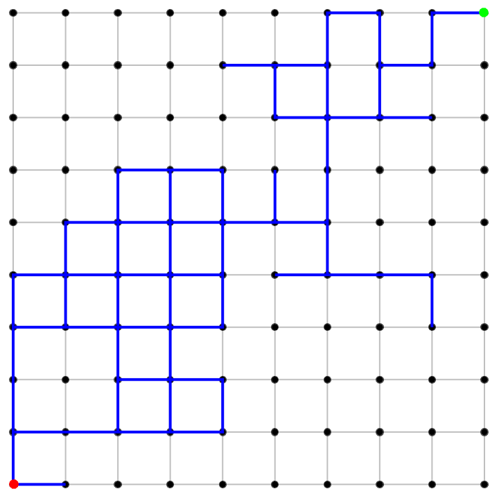
Manipulate[
 Module[
  {gridDims = {mazeSize, mazeSize, mazeSize}, mazeGraph, spanningTree,
    vertexList3D, hallwayThickness = 0.3, mazeRegion, inMazeQ,
   mazeSegments, chosenCorrMat, chol, positions, velocities, paths,
   stepCount, colorFunc, finalViewPoint, cubes},
  mazeGraph = GridGraph[gridDims, EdgeWeight -> (_ :> RandomReal[])];
  spanningTree = FindSpanningTree[mazeGraph];
  vertexList3D =
   AssociationThread[
    VertexList[mazeGraph] ->
     Map[Function[
       i, {Mod[i - 1, gridDims[[1]]] + 1,
        Mod[Floor[(i - 1)/gridDims[[1]]], gridDims[[2]]] + 1,
        Floor[(i - 1)/(gridDims[[1]]*gridDims[[2]])] + 1}],
      VertexList[mazeGraph]]];
  With[
   {edges = List @@@ EdgeList[spanningTree]},
   mazeSegments = Map[Line[vertexList3D /@ #] &, edges];
   mazeRegion = RegionUnion[
     RegionDilation[
      DiscretizeGraphics[
       Graphics3D[mazeSegments]],
      Ball[{0, 0, 0}, hallwayThickness]],
     Cuboid[{hallwayThickness, hallwayThickness, hallwayThickness},
      gridDims + 1 - hallwayThickness]];];
  inMazeQ = RegionMember[mazeRegion];
  cubes = Flatten[
    Table[{
      Opacity[0.025, Yellow],
      Cuboid[{x - 0.2, y - 0.2, z - 0.2},
       {x + 0.2, y + 0.2, z + 0.2}]},
     {x, gridDims[[1]]}, {y, gridDims[[2]]}, {z, gridDims[[3]]}], 2];
  chosenCorrMat = Switch[
    correlationChoice, "Independent", IdentityMatrix[3], "Moderate",
    {{1, 0.5, 0.3}, {0.5, 1, 0.4}, {0.3, 0.4, 1}}, "Strong",
    {{1, 0.9, 0.8}, {0.9, 1, 0.85}, {0.8, 0.85, 1}}, "Quantum",
    {{1, 0.8, 0.5}, {0.8, 1, 0.6}, {0.5, 0.6, 1}}, "DrillTeam",
    {{1, 0.9, 0.7}, {0.9, 1, 0.75}, {0.7, 0.75, 1}}, "Custom",
    {{1, xyCorr, xzCorr}, {xyCorr, 1, yzCorr}, {xzCorr, yzCorr,
      1}}, _, IdentityMatrix[3]];
  chol = Quiet@Check[
     CholeskyDecomposition[chosenCorrMat], None];
  If[chol === None, Return[
     Style["Invalid correlation matrix. Check that it is PSD.", Red,
      14]];];
  stepCount = maxSteps;
  positions = ConstantArray[
    initPos, particleCount];
  paths = Table[
    ConstantArray[initPos, stepCount], {particleCount}];
  Do[velocities = Transpose[
     chol .
      Transpose[
       RandomVariate[
        NormalDistribution[0, movementVariance], {particleCount, 3}]]];
   positions += velocities*timeDelta;
   positions = Table[
     If[inMazeQ[positions[[idx]]], positions[[idx]],
      positions[[idx]] - velocities[[idx]]*timeDelta], {idx,
      particleCount}];
   paths[[All, s]] = positions;, {s, 2, stepCount}];
  colorFunc = ColorData["Rainbow"];
  finalViewPoint = Switch[
    viewpointChoice, "Front", {0, -1, 0},
    "Top", {0, 0, 1},
    "Left", {-1, 0, 0},
    "Right", {1, 0, 0},
    "RotateView",
    Dynamic[
     RotationMatrix[
       rotationAngle, {0, 0, 1}] . {
       3, -3, 2}], _, {3, -3, 2}];
  Graphics3D[
   {{Opacity[0.1, Cyan], mazeRegion},
    cubes,
    Table[{colorFunc[i/particleCount],
      Tube[paths[[i, ;; displayStep]], 0.05],
      Sphere[paths[[i, displayStep]], 0.12]}, {i, particleCount}],
    {Green, Sphere[initPos, 0.2],
     Text[Style["Start", 14], initPos + {0, 0, -0.7}]},
    {Red, Cuboid[gridDims + 0.5],
     Text[Style["Exit", 14], gridDims + {0.5, 0.5, 1}]}},
   PlotRange -> {{0, mazeSize + 1}, {0, mazeSize + 1}, {0,
      mazeSize + 1}}, SphericalRegion -> True, Boxed -> True,
   Lighting -> "Neutral", ImageSize -> Large,
   ViewPoint -> finalViewPoint, Epilog -> {
     Inset[Framed@MatrixForm[
        N[chosenCorrMat, 3],
        TableDirections -> {Column, Row}],
      Scaled[{0.8, 0.2}]]}]],
 {{displayStep, 1, "Simulation Time Step"}, 1, maxSteps, 1,
  Appearance -> "Labeled"}, {{mazeSize, 8, "Maze Dimension"}, 4, 12,
  1, Appearance -> "Labeled"}, {{particleCount, 15,
   "Number of Particles"}, 1, 100, 1,
  Appearance -> "Labeled"}, {{maxSteps, 500, "Max Steps"}, 50, 1000,
  50, Appearance -> "Labeled"},
 {{timeDelta, 1, "Time Delta"}, 0.01, 1, 0.01,
  Appearance -> "Labeled"}, {{movementVariance, 0.15,
   "Movement Variance (\[Sigma])"}, 0.01, 1, 0.01,
  Appearance -> "Labeled"}, {{correlationChoice, "Independent",
   "Correlation Type"}, {"Independent", "Moderate", "Strong",
   "Quantum", "DrillTeam", "Custom" -> "Custom"}},
 Control@{{xyCorr, 0.0, "X-Y Corr."}, -1, 1, 0.1,
   Appearance -> "Labeled",
   Enabled -> Dynamic[correlationChoice === "Custom"]},
 Control@{{xzCorr, 0.0, "X-Z Corr."}, -1, 1, 0.1,
   Appearance -> "Labeled",
   Enabled -> Dynamic[correlationChoice === "Custom"]},
 Control@{{yzCorr, 0.0, "Y-Z Corr."}, -1, 1, 0.1,
   Appearance -> "Labeled",
   Enabled ->
    Dynamic[correlationChoice === "Custom"]}, {{viewpointChoice, "3D",
    "View Angle"},
  {"Front", "Top", "Left", "Right", "3D" -> "3D",
   "RotateView" -> "RotateView"}}, {{rotationAngle, 0,
   "Rotation Angle"},
  0, 2 Pi, 0.02, Appearance -> "Labeled",
  Enabled -> Dynamic[viewpointChoice === "RotateView"]},
 {{initPos, {1.5, 1.5, 1.5}, "Initial Position (x,y,z)"},
  InputField},
 SynchronousUpdating -> False,
 TrackedSymbols :> {displayStep, mazeSize, correlationChoice,
   xyCorr, xzCorr, yzCorr, movementVariance, viewpointChoice,
   rotationAngle, maxSteps, timeDelta, particleCount, initPos,
   chosenCorrMat}]
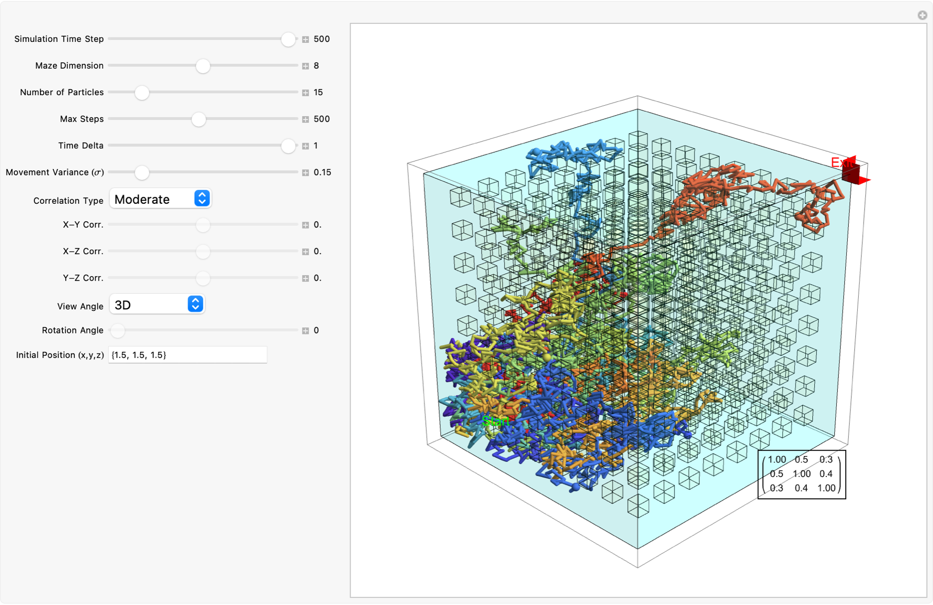
I mean, the exploration of randomness in computational pathfinding and the beauty of "dumb" solutions that, paradoxically, work..show how a maze could be "solved" simply by letting a host of particles follow Brownian motion until one--by sheer luck--finds the exit. My idea is that I'm going to let a gas go here and then at some point one of the atoms of the gas is going to reach the exit. You can always find some element of computational irreducibility; if you let enough particles wander freely within a well-defined maze (constructed, for example, via a spanning tree over a grid), one of them is bound to take the right turns and eventually escape; we can construct an obstacle like a stick of butter for instance, and then when the particles encounter the obstacle they get an emergent reward; after a while, this is the one that's going to end up winning; it got out there "first", via our correlation matrix..and this is the path that it took the whole time. By highlighting the eventual dominance of the winning trajectory, we don't even "know what a mathematician is"; once we refine our code so that once the winning condition is detected--whether by a particle inadvertently crossing a defined exit boundary or reaching a threshold--the simulation fades out all other paths. But more importantly, this spotlighting of the winning route not only improves clarity but reinforces a broader metaphor about what we're missing out on; there's just this massive flood of randomness, and amid this sea of randomness one path is destined to emerge. You know what it reminds me of? Sperm going to the egg. Which sperm will become a human? Just as countless sperm compete with no predetermined plan--only to have one succeed in fertilization--so too do our simulated particles "compete" in the maze. Even though e-very molecule acts without foresight, the circuitous unpredictability occasionally yields a serendipity, that shapes success in nature and business; everybody is just bumping around randomly--but the one person you know who became a billionaire? It wasn't due to some grand plan; it was just random. The more you expose kids to the realities of money, the better they'll understand its true value--from the cost of a car to the price of a house. There might be the most efficient way to do something but, hey, this works. And maybe it's not the dumbest way because it does work, right? Amid all the contributors knocking, doing things the beauty of our maze solver lies in its simplicity. Instead of building an algorithm with heuristics, we allow random walks to do the heavy lifting. In the future, the line between human relationships and relationships with Artificial Intelligence will blur; these systems may know more about us than we know ourselves. Humanoid robots aren't just science fiction--they'll become integral to our world, precisely because our environment is designed for the human form. How can I make it..you could either write all the code to solve this maze or just release a bad smell; sometimes a simple, "dumb" approach gets the job done. This is a lesson not only in computational creativity but also in the elegance of our metaphor of water particles causing not only a massive amount of damage but also leading us to the elegance of emergent behavior. But I can only explain so much in words. Without further ado, let's introduce some correlation matrices so we can prepare for some futuristic "string-tightening" optimization which yields a path that is both feasible and near-optimal.
SeedRandom[1234];
dims = {8, 8, 8};
mazeGraph = GridGraph[
   dims, EdgeWeight -> (_ :> RandomReal[])];
spanningTree = FindSpanningTree[
   mazeGraph];
vertexCoords = Flatten[
   Table[{i, j, k}, {i, dims[[1]]}, {j, dims[[2]]}, {k, dims[[3]]}],
   2];
nodeCoords = AssociationThread[
   VertexList[mazeGraph], vertexCoords];
pathSegments = Line[
     Lookup[nodeCoords, #]] & /@ EdgeList[spanningTree];
hallwayThickness = 0.3;
mazeBaseRegion = RegionUnion[
   RegionDilation[
    DiscretizeGraphics[
     Graphics3D[pathSegments]
     ],
    Ball[{0, 0, 0}, hallwayThickness]
    ],
   Cuboid[
    {hallwayThickness, hallwayThickness, hallwayThickness},
    dims + 1 - hallwayThickness]];
numObstacles = 1;
obstacleSize = {8, 2, 2};
obstacleRegionList = Table[
   Module[{pos},
    pos = {RandomReal[{hallwayThickness,
        dims[[1]] + 1 - obstacleSize[[1]] - hallwayThickness}],
      RandomReal[{hallwayThickness,
        dims[[2]] + 1 - obstacleSize[[2]] - hallwayThickness}],
      RandomReal[{hallwayThickness,
        dims[[3]] + 1 - obstacleSize[[3]] - hallwayThickness}]};
    Cuboid[pos, pos + obstacleSize]], {numObstacles}];
mazeRegion =
  RegionDifference[mazeBaseRegion,
   RegionUnion @@ obstacleRegionList];
teleportTarget = {
   dims[[1]] + 1 - hallwayThickness,
   hallwayThickness,
   (dims[[1]] + 1 - hallwayThickness) / 1.1};
particleCount = 3;
initPos = {1.5, 1.5, 1.5};
maxSteps = 1500;
timeStep = 0.00115;
simulateParticles[chol_?MatrixQ, noiseScale_] := Module[
   {positions, paths, inMazeQ, vel, newPos, subdivisions = 10,
    obstacleQ}, inMazeQ = RegionMember[mazeRegion];
   obstacleQ[pt_] :=
    Or @@ (RegionMember[#, pt] & /@ obstacleRegionList);
   positions = ConstantArray[initPos, particleCount];
   paths = Table[
     ConstantArray[initPos, maxSteps],
     {particleCount}];
   clearPath[oldPos_, newPos_] := Module[
     {points},
     points =
      Table[oldPos + (newPos - oldPos)*(i/subdivisions), {i, 1,
        subdivisions}];
     AllTrue[points, inMazeQ]];
   Do[
    Do[vel =
      noiseScale*(chol . RandomVariate[NormalDistribution[0, 1], {3}]);
     newPos = positions[[j]] + vel*timeStep;
     If[clearPath[positions[[j]], newPos],
      positions[[j]] = newPos,
      If[obstacleQ[newPos], positions[[j]] = teleportTarget,
       positions[[j]] = positions[[j]] - vel*timeStep]
      ];, {j, particleCount}];
    Do[
     paths[[k, i]] = positions[[k]],
     {k, particleCount}
     ];,
    {i, 2, maxSteps}];
   paths];
axisMarkers = {
   {Red, Arrow[{{0, 0, 0}, {3, 0, 0}}],
    Text[Style["X", Bold, 14, Red], {3.2, 0, 0}]},
   {Green, Arrow[{{0, 0, 0}, {0, 3, 0}}],
    Text[Style["Y", Bold, 14, Green], {0, 3.2, 0}]},
   {Blue, Arrow[{{0, 0, 0}, {0, 0, 3}}],
    Text[Style["Z", Bold, 14, Blue], {0, 0, 3.2}]}};
DynamicModule[
 {simPaths, newSim = True},
 Manipulate[
  Module[
   {chol, plotRange},
   chol =
    Quiet[Check[
      CholeskyDecomposition[{{xx, xy, xz}, {xy, yy, yz}, {xz, yz,
         zz}}], IdentityMatrix[3]]];
   If[newSim,
    simPaths = simulateParticles[chol, noiseScale];
    newSim = False];
   plotRange = {
     {0, dims[[1]] + 1},
     {0, dims[[2]] + 1},
     {0, dims[[3]] + 1}};
   Graphics3D[
    {{Opacity[0.2, LightBlue], mazeRegion},
     {Opacity[0.5, Darker[Gray, 0.2]], obstacleRegionList},
     Table[
      {
       ColorData["Rainbow"][n/particleCount],
       Tube[
        Take[simPaths[[n]], Min[step, Length[simPaths[[n]]]]],
        0.05],
       Sphere[simPaths[[n, Min[step, Length[simPaths[[n]]]]]], 0.1]},
      {n, particleCount}],
     {Green, Sphere[initPos, 0.2]},
     {Black,
      Text[Style["EXIT", Bold, 14, White], dims + {0.5, 0.5, 0.5}]},
     axisMarkers},
    PlotRange -> plotRange,
    Boxed -> True,
    Lighting -> "Neutral",
    ImageSize -> 800,
    SphericalRegion -> True,
    ViewPoint -> {3 Cos[\[Theta]], 3 Sin[\[Theta]], 2},
    PlotLabel ->
     Style["Correlation Matrix:\n" <>
       ToString[
        MatrixForm[{{xx, xy, xz}, {xy, yy, yz}, {xz, yz, zz}}]],
      White, Bold]]], {{step, 1, "Step"}, 1, maxSteps, 1,
   Appearance -> "Labeled"},
  {{\[Theta], 0, "View Rotation (\[Theta])"}, 0, 2 Pi,
   Appearance -> "Labeled"},
  Delimiter, {{xx, 1, "X-X Correlation"}, 0, 1, 0.1,
   Appearance -> "Labeled"},
  {{xy, -1, "X-Y Correlation"}, -1, 1, 0.1, Appearance -> "Labeled"},
  {{xz, -1, "X-Z Correlation"}, -1, 1, 0.1, Appearance -> "Labeled"},
  {{yy, 1, "Y-Y Correlation"}, 0, 1, 0.1, Appearance -> "Labeled"},
  {{yz, -1, "Y-Z Correlation"}, -1, 1, 0.1, Appearance -> "Labeled"},
  {{zz, 1, "Z-Z Correlation"}, 0, 1, 0.1, Appearance -> "Labeled"},
  Delimiter, {{noiseScale, 200, "Noise Scale"}, 1, 200, 20,
   Appearance -> "Labeled"},
  Delimiter,
  Button["New Simulation (after changing sliders)", newSim = True;],
  TrackedSymbols :> {step, \[Theta], xx, xy, xz, yy, yz, zz,
    noiseScale, newSim},
  SynchronousUpdating -> False]]
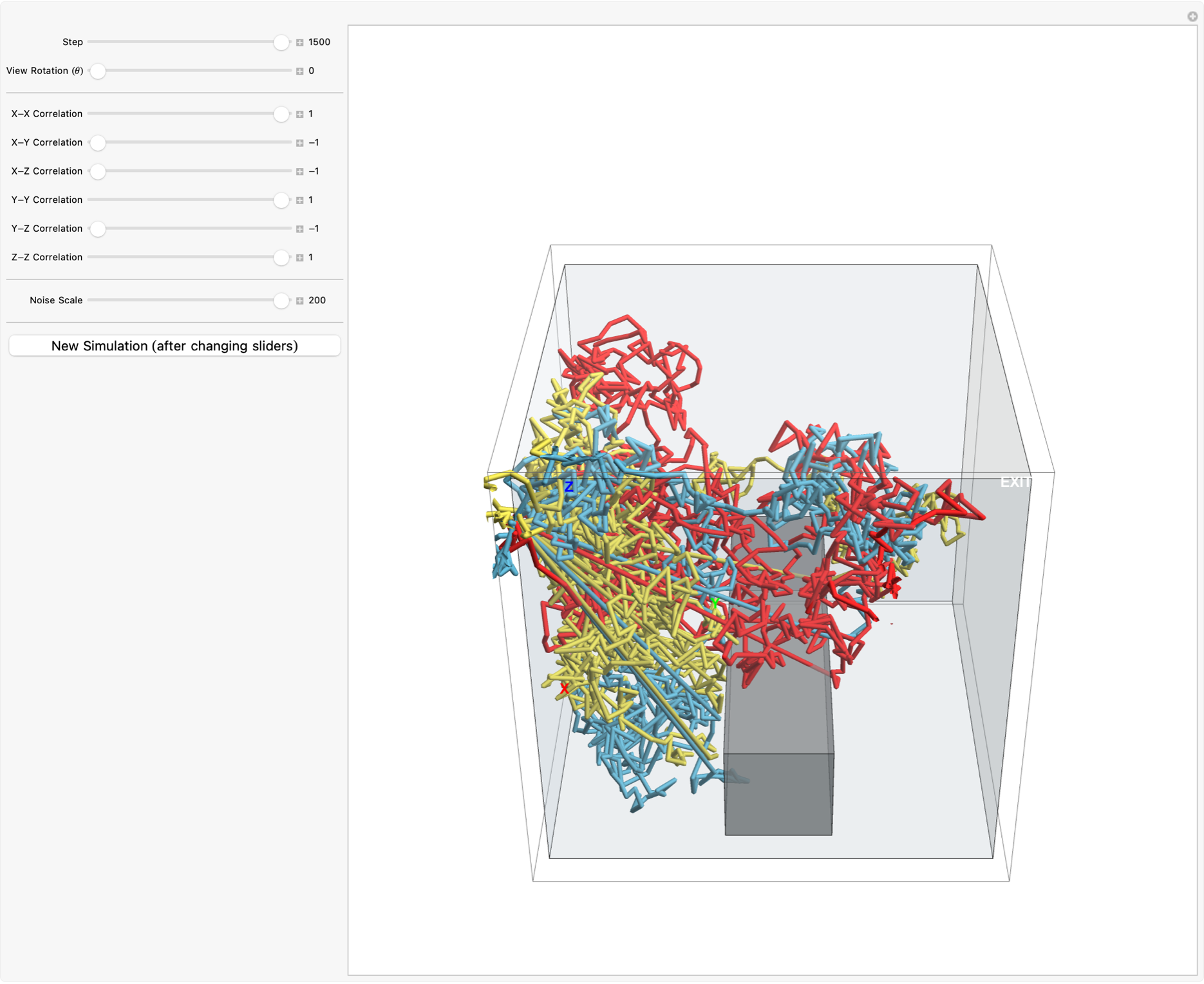
There's a certain kind of reality distortion that you need to have if you're gonna go out and do something bold. When a particle eventually barges through and reaches the obstacle, it's teleported onto a greater location. This particle, has proverbially left the station because it's, with a "helpful" nudge we can re-introduce inter-particle interactions, or we could..get this razor thin definition where the particles are occasionally able to cross through the obstacle. And then the particles are left within the test function self signature. Right now and throughout the "time steps" we can visualize, the way that our maze solving methodology warms up with the optimum correlation matrix. Our Brownian Motion Maze Solving, conveniently corroborates our belief system about how when a particle approaches an obstacle, it's not because there's something fundamentally wrong with it--it might simply be because as it happens, it takes about a two-week period to prove that what seems impossible can actually work if you commit to it. What seems like a Ruliad of infinite possibilities, we're left with a dim awareness that knowing what could go wrong tells you exactly how far the ground is if you fall--this clarity gives me the confidence to take risks. Each project is an opportunity to invest in something; always invest in what you understand--and if you love and use a company's product, that's a strong signal it's worth backing. Case in point, the same way that we do these two-week projects, is the same way I'm going to let a gas go here and then at some point one of the atoms of the gas is going to reach the exit. So if we ever change our mind about the most efficient way to do something, we'll realize that after a while, this is the one that's going to end up winning; it got out there first, and this is the path that it took the whole time. That is why Brownian Motion Maze Solving explains the element of conviction, that the contiguous path our particles take reflects a recurring theme that chance can be as potent a mechanism as any engineered algorithm.


