Message Boards Message Boards

0
|
6205 Views
|
6 Replies
|
3 Total Likes
View groups...
Share
Share this post:

Probability density of a Cos function for Normal variable?

Posted 1 year ago

Hello

I am reading the Wikipedia article about the normal distribution (section Operations and functions of normal variables), and I am unable to obtain with Mathematica the first example given, namely:

Probability density of the function cos( x^2) of a normal variable x with μ = − 2 and σ = 3 .

PDF cannot be of help as it applies to a distribution of a variable and not to a function of a variable whose distribution is normal, and I do know not other Mathematica functions to compute probability density.

Thanks.

POSTED BY: Jan Potocki
6 Replies
Posted 1 year ago

For whatever it's worth the second answer followed what's done for a "wrapped normal" distribution.

For the first answer, I chose a 1-to-1 formula and Abs[xx] is not 1-to-1.

POSTED BY: Jim Baldwin
Posted 1 year ago

Thanks Jim for your second answer which is thorough and well explained., A solution to get inspiration from when the function TransformedDistribution does not work.

In your first answer could you comment more on the way you choose to scale xx to be between 0 and 1 ? Why the simpler Abs[xx] is not suitable ? I tried that with a smaller sample but the result obtained afterwards is wrong..

POSTED BY: Jan Potocki
Posted 1 year ago

Here is an approach the results in an explicit answer for the pdf of $\cos(X^2)$ where $X$ has a normal distribution with mean $\mu$ and variance $\sigma^2$.

The pdf has an infinite number of terms but can be approximated well with a finite number of terms.

First solve for $x$ in $Cos[x^2]==c$:

Solve[Cos[x^2] == c, x]

Solutions for x

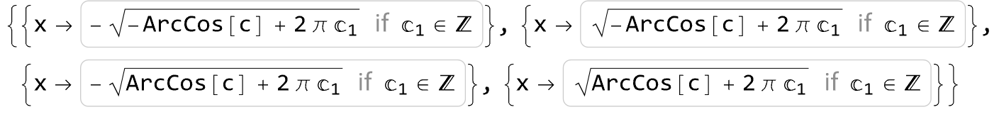
We see that there are a infinite number of values of $x$ that give the same value of $\cos(x^2)$. We need to make sure we account for all of those so that we can add up all of the contributions from the pdf of
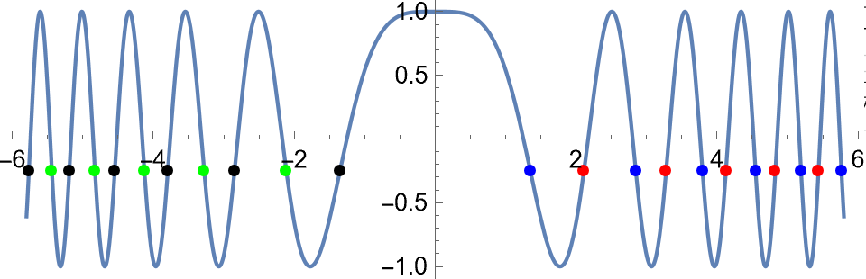
 $X$. Consider $c=-0.4$:

c0 = -1/4;
Show[Plot[Cos[x^2], {x, -5.8, 5.8}],
  ListPlot[Table[{-Sqrt[-ArcCos[c] + 2 \[Pi] k], c} /. c -> c0, {k, 1, 5}], PlotStyle -> Green],
  ListPlot[Table[{Sqrt[-ArcCos[c] + 2 \[Pi] k], c} /. c -> c0, {k, 1, 5}], PlotStyle -> Red],
  ListPlot[Table[{-Sqrt[ArcCos[c] + 2 \[Pi] k], c} /. c -> c0, {k, 0, 5}], PlotStyle -> Black],
  ListPlot[Table[{Sqrt[ArcCos[c] + 2 \[Pi] k], c} /. c -> c0, {k, 0, 5}], PlotStyle -> Blue],
  AspectRatio -> 1/3]

Plot of cos(x^2) and values of x where c=-0.4

So for a particular value of c we add up all of the associated density values multiplied by the absolute value of the corresponding Jacobian to obtain the contributions. First the Jacobians:

j1 = D[-Sqrt[-ArcCos[c] + 2 \[Pi] k], c] // Abs
(* 1/2 Abs[1/(Sqrt[1-c^2] Sqrt[2 k \[Pi]-ArcCos[c]])] *)
j2 = D[Sqrt[-ArcCos[c] + 2 \[Pi] k], c] // Abs
(* 1/2 Abs[1/(Sqrt[1-c^2] Sqrt[2 k \[Pi]-ArcCos[c]])] *)
j3 = D[-Sqrt[ArcCos[c] + 2 \[Pi] k], c] // Abs
(* 1/2 Abs[1/(Sqrt[1-c^2] Sqrt[2 k \[Pi]+ArcCos[c]])] *)
j4 = D[Sqrt[ArcCos[c] + 2 \[Pi] k], c] // Abs
(* 1/2 Abs[1/(Sqrt[1-c^2] Sqrt[2 k \[Pi]+ArcCos[c]])] *)

Now for the pdf of $\cos(X^2)$:

pdf[c_, \[Mu]_, \[Sigma]_, kmax_] :=
 Sum[j1 PDF[NormalDistribution[\[Mu], \[Sigma]], -Sqrt[-ArcCos[c] + 2 \[Pi] k]], {k, 1, kmax}] +
  Sum[j2 PDF[NormalDistribution[\[Mu], \[Sigma]], Sqrt[-ArcCos[c] + 2 \[Pi] k]], {k, 1, kmax}] +
  Sum[j3 PDF[NormalDistribution[\[Mu], \[Sigma]], -Sqrt[ArcCos[c] + 2 \[Pi] k]], {k, 0, kmax}] +
  Sum[j4 PDF[NormalDistribution[\[Mu], \[Sigma]], Sqrt[ArcCos[c] + 2 \[Pi] k]], {k, 0, kmax}]

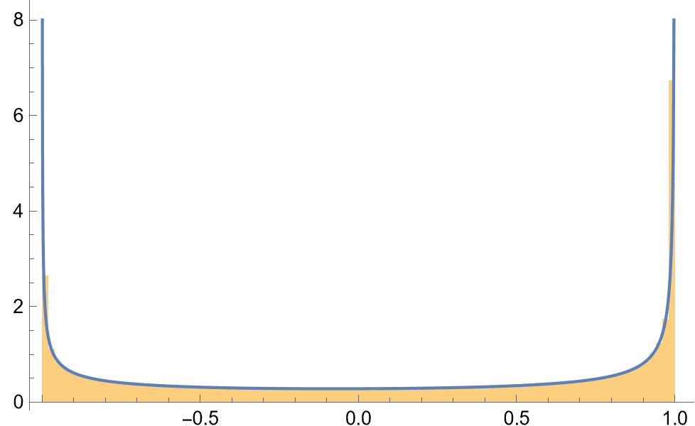
We can check this out with a finite number of terms (i.e., setting kmax to 50 rather than $\infty$:

SeedRandom[12345];
n = 1000000;
cc = Cos[RandomVariate[NormalDistribution[-2, 3], n]^2];

Show[Histogram[cc, "FreedmanDiaconis", "PDF"],
 Plot[pdf[c, -2, 3, 100], {c, -1, 1}, PlotRange -> {{-1, 1}, {0, 8}}]]

pdf of cos(x^2)

POSTED BY: Jim Baldwin
Posted 1 year ago

The closed-form solution for this probability density is in the eye of the beholder as it is expressed with an infinite number of terms.

$$\sum _{k=1}^{\infty} \frac{e^{-\frac{1}{18} \left(2-\sqrt{2 \pi k-\cos ^{-1}(c)}\right)^2}}{6 \sqrt{2 \pi } \sqrt{1-c^2} \sqrt{2 \pi k-\cos ^{-1}(c)}}+\sum _{k=1}^{\infty} \frac{e^{-\frac{1}{18} \left(\sqrt{2 \pi k-\cos ^{-1}(c)}+2\right)^2}}{6 \sqrt{2 \pi } \sqrt{1-c^2} \sqrt{2 \pi k-\cos ^{-1}(c)}}+\sum _{k=0}^{\infty} \frac{e^{-\frac{1}{18} \left(2-\sqrt{\cos ^{-1}(c)+2 \pi k}\right)^2}}{6 \sqrt{2 \pi } \sqrt{1-c^2} \sqrt{\cos ^{-1}(c)+2 \pi k}}+\sum _{k=0}^{\infty} \frac{e^{-\frac{1}{18} \left(\sqrt{\cos ^{-1}(c)+2 \pi k}+2\right)^2}}{6 \sqrt{2 \pi } \sqrt{1-c^2} \sqrt{\cos ^{-1}(c)+2 \pi k}}$$

but a good approximation can be had with 40 to 50 terms per summation.

Here is the Mathematica code:

kmax =.
pdf =
 Sum[PDF[NormalDistribution[-2, 3], Sqrt[ArcCos[c] + 2 \[Pi] k]] 1/(2 Sqrt[1 - c^2] Sqrt[2 k \[Pi] + ArcCos[c]]), {k, 0, kmax}] +
  Sum[PDF[NormalDistribution[-2, 3], Sqrt[-ArcCos[c] + 2 \[Pi] k]] 1/(2 Sqrt[1 - c^2] Sqrt[2 k \[Pi] - ArcCos[c]]), {k, 1, kmax}] +
  Sum[PDF[NormalDistribution[-2, 3], -Sqrt[ArcCos[c] + 2 \[Pi] k]] 1/(2 Sqrt[1 - c^2] Sqrt[2 k \[Pi] + ArcCos[c]]), {k, 0, kmax}] +
  Sum[PDF[NormalDistribution[-2, 3], -Sqrt[-ArcCos[c] + 2 \[Pi] k]] 1/(2 Sqrt[1 - c^2] Sqrt[2 k \[Pi] - ArcCos[c]]), {k, 1, kmax}]

I'll put in the details sometime soon.

POSTED BY: Updating Name
Posted 1 year ago

As Eric Rimbey mentions TransformedDistribution is the function to try. However, in this case Mathematica does not find a pdf (and a closed-form might not even exist).

The next thing to try is to take a large sample and look at the resulting shape of the distribution. In this case, it appears that a beta distribution might provide a good fit (but properly scaled to have values between -1 and 1).

dist = TransformedDistribution[Cos[x^2], x \[Distributed] NormalDistribution[-2, 3]];
xx = RandomVariate[dist, 10000000];

(* Scale xx to be between 0 and 1 *)
z = (1 + xx)/2;

(* Solve for the corresponding moments of a beta distribution *)
sol = Solve[{Mean[z] == Mean[BetaDistribution[a, b]],
    Variance[z] == Variance[BetaDistribution[a, b]]}, {a, b}][[1]]
(* {a -> 0.485618, b -> 0.369652} *)

(* Show results *)
Show[Histogram[xx, "FreedmanDiaconis", "PDF"],
 Plot[PDF[BetaDistribution[a, b] /. sol, (1 + x)/2]/2, {x, -1, 1}, PlotRange -> {{0.01, 0.99}, {0, 8}}]]

Beta distribution fitted with method of moments

POSTED BY: Jim Baldwin
Posted 1 year ago

I think you might be able to use TransformedDistribution.

POSTED BY: Eric Rimbey
Reply to this discussion
Community posts can be styled and formatted using the Markdown syntax.
Reply Preview
Attachments
Remove
or Discard

Group Abstract Group Abstract