Even though chess is much too difficult to analyze by comprehensive combinatorics, it's at least a relatively simple game in terms of implements. A typical chess set has only 32 pieces in six classes and two colors. Those pieces move on a flat board, which is really just an 8$\times$8 array (and 2-colored with an alternating pattern). Since electronic games draw maps from a hidden memory store, they are usually much more difficult to interpret. The purpose of this memo is to extract a height map from isomorphic pixel data using the Classify function (part of built-in WL machine learning capabilities).
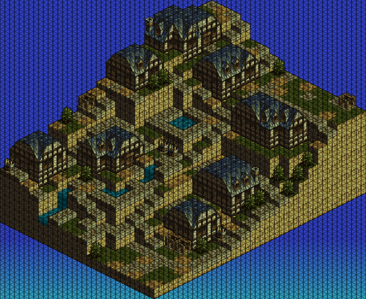
SNES maps as a data set can be described as pixel grids of arbitrary size, with 256 on-screen colors, already much more complicated than chess. As a particular example, let's take the newly re-released game Tactics Ogre (1995), a genre-defining adaptation of table-top RPG mechanics to a digital medium. Scenario maps are depicted in isomorphic view, as m$\times$n grids with an extra added height dimension. The extra height dimension is what can really make a scenario more interesting, because height differences constrain motion of the characters. This potentially gives advantage to characters with better jump statistics (kunoichi) or with ranged attacks (archers, mages).
We can start graphical analysis by importing a map as data and checking its ImageDimensions:
im1=Import[
 "https://www.vgmaps.com/Atlas/SuperNES/TacticsOgre-LetUsClingTogether(J)-Griate-Chapter2-ChaoticBattle&Training(Unmarked).png"];
ImageDimensions@im1
ImageDimensions[im1]/{32, 16}

Out[] = {608, 496}
Out[] = {19, 31}
This gives us an idea that the isomorphic grid is built up from blocks of size $16\times 32$, which can be triangulated as follows:
Row[Show[#, ImageSize -> 200] & /@ {ArrayPlot[Table[If[Or[
       MemberQ[{16, 17, -15, -16}, 2 i - j],
       MemberQ[{17, 18, 49, 50}, 2 i + j]
       ], 1, 0], {i, 1, 16}, {j, 1, 32}]], ArrayPlot[Table[If[Or[
       MemberQ[{1, 8, 9, 16, 17, 24, 25, 32}, j],
       MemberQ[{0, 1, 16, 17, -15, -16}, 2 i - j],
       MemberQ[{17, 18, 33, 34, 49, 50}, 2 i + j]
       ], 1, 0], {i, 1, 16}, {j, 1, 32}]]}, Spacer[20]]
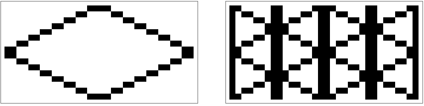
The first image depicts what is basically a chess-square viewed from an isomorphic perspective, and the second image accounts for possibly half-length offsets. In subsequent calculations, to go up half-steps or even just to move between adjacent squares, we will need to use actions of a Klein four group to switch between four distinct ImagePartition's. Here's what we get by applying the triangularization to the source image:
ImageAdd[ImageMultiply[im1, pixelGrid], ImageMultiply[
  1/2*ColorNegate@ArrayPlot[ArrayFlatten[ConstantArray[Table[If[Or[
          MemberQ[{1, 8, 9, 16, 17, 24, 25, 32}, j],
          MemberQ[{0, 1, 16, 17, -15, -16}, 2 i - j],
          MemberQ[{17, 18, 33, 34, 49, 50}, 2 i + j]
          ], 1, 0], {i, 1, 16}, {j, 1, 32}], {31, 19}]],
     Frame -> False, PixelConstrained -> 1], im1]]
We would like to use this map to train a ClassifierFunction via Classify, so we need to manually enter a data set describing the location of various objects on screen and their relative heights:
golyatData = Association[{
    "Heights" -> {
      {11, 9, 9, 9, 11, 15, 15, 15, 16, 18, 19, 19, 19, 19, 22, 20,
       20, 20, 20, 24, 24, 24},
      {11, 9, 9, 9, 11, 15, 15, 15, 16, 17, 19, 19, 19, 19, 22, 20,
       20, 20, 20, 20, 24, 24},
      {10, 9, 9, 9, 11, 12, 13, 14, 14, 14, 19, 19, 19, 19, 22, 22,
       20, 20, 20, 20, 24, 24},
      {9, 9, 10, 10, 10, 10, 10, 10, 10, 14, 19, 19, 19, 19, 19, 20,
       20, 20, 21, 21, 22, 23},
      {5, 5, 8, 9, 9, 10, 10, 10, 10, 13, 13, 14, 14, 14, 18, 18, 16,
       16, 16, 16, 20, 20},
      {6, 6, 9, 9, 9, 10, 10, 10, 10, 12, 13, 14, 13, 13, 14, 17, 16,
       16, 16, 16, 20, 20},
      {5, 5, 8, 9, 8, 10, 10, 10, 11, 11, 11, 14, 13, 13, 14, 16, 16,
       16, 16, 16, 18, 19},
      {5, 6, 7, 9, 8, 8, 9, 8, 10, 11, 11, 14, 14, 14, 14, 15, 16, 17,
        17, 17, 17, 17},
      {5, 5, 5, 9, 9, 9, 9, 9, 11, 11, 10, 11, 12, 13, 14, 15, 16, 17,
        17, 17, 17, 17},
      {2, 2, 5, 5, 6, 7, 8, 9, 9, 9, 9, 9, 9, 9, 13, 13, 13, 13, 17,
       17, 17, 17},
      {2, 2, 2, 2, 5, 5, 6, 6, 6, 6, 5, 5, 5, 9, 13, 13, 13, 13, 17,
       17, 17, 17},
      {2, 2, 2, 2, 3, 4, 2, 2, 2, 6, 5, 5, 5, 9, 13, 13, 13, 13, 17,
       17, 17, 17},
      {2, 2, 2, 2, 2, 2, 2, 2, 2, 6, 5, 5, 5, 9, 13, 13, 13, 13, 17,
       17, 17, 17},
      {2, 2, 2, 2, 2, 2, 2, 2, 2, 5, 5, 5, 5, 9, 13, 13, 13, 13, 17,
       17, 17, 17},
      {2, 2, 2, 2, 2, 2, 2, 2, 3, 4, 5, 6, 6, 8, 9, 13, 13, 13, 17,
       17, 17, 17},
      {2, 2, 2, 2, 2, 2, 2, 2, 3, 4, 5, 6, 6, 7, 7, 9, 11, 14, 16, 17,
        17, 17}
      },
    "Barrels" -> {
      {1, 1}, {7, 11}, {8, 11}, {15, 9}
      },
    "Crates" -> {
      {1, 9}, {14, 6}, {13, 6}, {15, 22}
      },
    "Bushes" -> {
      {1, 7}, {4, 13}, {4, 14}, {5, 5}, {10, 1},
      {15, 7}, {15, 12}, {15, 13}, {15, 15},
      {16, 15}, {16, 16}, {16, 17}, {8, 22}
      },
    "Water" -> {
      {5, 1}, {5, 2}, {5, 3}, {7, 5},
      {8, 5}, {8, 6}, {8, 8}, {8, 9},
      {6, 13}, {6, 14}, {7, 13}, {7, 14}
      },
    "Houses" -> Association[{
       "Lower" -> Association[{

          3 -> {{1, 12}, {1, 13}, {1, 14}, {2, 12}, {2, 13}, {2,
             14}, {3, 12},
            {3, 13}, {3, 14}, {4, 6}, {4, 7}, {4, 8}, {4, 9}, {5,
             6}, {5, 7},
            {5, 8}, {5, 9}, {6, 7}, {6, 8}, {6, 9}},

          4 -> {{12, 7}, {12, 8}, {12, 9}, {13, 7}, {13, 8}, {13,
             9}, {14, 7},
            {14, 8}, {14, 9}, {11, 11}, {11, 12}, {11, 13}, {12,
             11}, {12, 12},
            {12, 13}, {13, 11}, {13, 12}, {13, 13}, {14, 11}, {14,
             12}, {14, 13},
            {10, 16}, {10, 17}, {10, 18}, {11, 16}, {11, 17}, {11,
             18}, {12, 16},
            {12, 17}, {12, 18}, {13, 16}, {13, 17}, {13, 18}, {14,
             17}, {14, 18},
            {5, 17}, {5, 18}, {5, 19}, {5, 20}, {6, 17}, {6, 18}, {6,
             19}, {6, 20},
            {7, 17}, {7, 18}, {7, 19}, {7, 20}, {1, 16}, {1, 17}, {1,
             18}, {1, 19},
            {2, 16}, {2, 17}, {2, 18}, {2, 19}, {2, 20}, {3, 17}, {3,
             18}, {3, 19}, {3, 20}},

          5 -> {{1, 2}, {1, 3}, {1, 4}, {2, 2}, {2, 3}, {2, 4}, {3,
             2}, {3, 3}, {3, 4}}
          }],
       "Upper" -> Association[{
          3 -> {{5, 8}, {6, 8}, {2, 12}, {2, 13}},
          4 -> {{13, 7}, {13, 8}, {14, 8},
            {13, 11}, {13, 12}, {13, 13},
            {12, 11}, {12, 12}, {12, 13},
            {11, 16}, {11, 17}, {12, 17},
            {6, 17}, {6, 18}, {6, 19},
            {1, 17}, {1, 18},
            {2, 17}, {2, 18}, {2, 19},
            {3, 18}, {3, 19}},
          5 -> {{2, 2}, {2, 3}, {3, 3}}
          }]
       }]
    }];
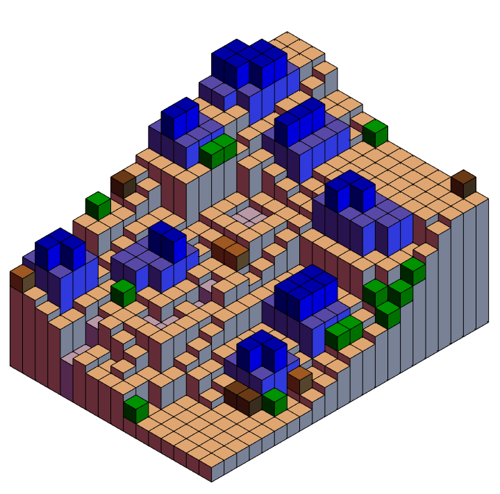
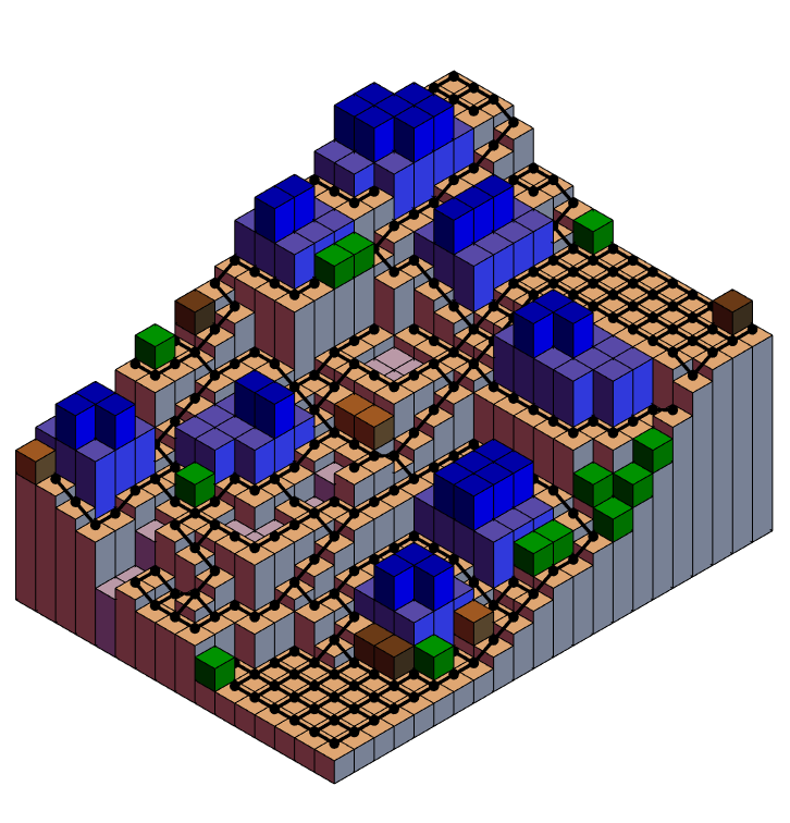
Ultimately we would like to have a machine learning function that goes from a map image, to extract data as written manually above. But we are about to see that even extracting the "Heights" is a not-entirely-trivial task that probably can't be accomplished from local texture information alone. Once we have such data, it's relatively easy to redraw the map in three dimensions:
base = With[{
    heightMap = golyatData["Heights"],
    water = golyatData["Water"]},
   Graphics3D[{MapIndexed[{
        If[MemberQ[water, #2],
         Lighter[Blue, 0.7],
         Lighter[Brown, 0.6]],
        Cuboid[Append[#2, 0], Append[#2 + {1, 1}, #1/2]]} &,
      heightMap, {2}]}, Boxed -> False, ViewVertical -> {0, 0, 1},
    ViewPoint -> {Infinity, -Infinity, Infinity}]];

obstructions = With[{heightMap = golyatData["Heights"]},
   Graphics3D[MapThread[Prepend, {Map[
       Cuboid[Append[#1, heightMap[[Sequence @@ #1]]/2],
         Append[#1 + {1, 1}, (heightMap[[Sequence @@ #1]] + 2)/2]] &,
       Lookup[golyatData, {"Crates", "Barrels", "Bushes"}], {2}],
      {Darker[Brown], Brown, Darker[Green]}}]]];

houses = Graphics3D[With[{heightMap = golyatData["Heights"]},
    Join[Map[Function[{height}, {Lighter@Blue, Map[
         Cuboid[Append[#1, heightMap[[Sequence @@ #1]]/2],

           Append[#1 + {1, 1}, (heightMap[[Sequence @@ #1]] + height)/
             2]] &,
         golyatData["Houses", "Lower", height]]}], {3, 4, 5}],
     Map[Function[{height}, {Blue, Map[
         Cuboid[Append[#1, (heightMap[[Sequence @@ #1]] + height)/2],

           Append[#1 + {1,
              1}, (heightMap[[Sequence @@ #1]] + height + 3)/2]] &,
         golyatData["Houses", "Upper", height]]}], {3, 4, 5}]]]];

Show[Show[base, obstructions, houses]]
And it's also possible to extract a states adjacency graph for a character who can't move on water and can only climb by one increment of height per step:
pathGraph = With[{heightMap = golyatData["Heights"],
   g1 = NearestNeighborGraph[Complement[
      Position[ConstantArray[1, {16, 22}], 1],
      Join[Catenate[Lookup[golyatData,
         {"Crates", "Barrels", "Bushes", "Water"}]],
       Catenate[Values[
         golyatData["Houses", "Lower"]]]]], {4, 1}]},
  Graph[Select[EdgeList[g1],
    Abs[Apply[Subtract, heightMap[[Sequence @@ #]] & /@ #]] < 2 &
    ], VertexCoordinates -> Map[
     # -> Times[Reverse[#], {1, -1}] &, VertexList[g1]]]
  ]
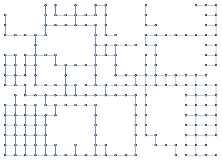
and overlay the graph on the map:
With[{heightMap = golyatData["Heights"]},
 Show[Show[base, obstructions, houses],
  Graph3D[pathGraph, VertexCoordinates -> Map[
     Append[# + {1/2, 1/2}, (heightMap[[Sequence @@ #]] + 1/2)/2] &,
     VertexList[pathGraph]], VertexStyle -> {Black}, EdgeStyle -> Black
   ]]]
With the height map known, we can also extract the set of $16\times32$ pixel arrays centered on squares where characters are allowed to stand and move through, as well as those that are obstructed by objects like crates, barrels, and bushes. We then can feed this data into Classify, and attempt to find subsequent height maps by an inductive process.
We need to compute slightly more data about four similar maps and their offsets:
sortedImageGrids = Association[MapThread[Rule, {
     Catenate[Outer[{#1 - 1, #2 - 1} &, {1, 2}, {1, 2}]],
     Catenate[Outer[ImagePartition[im1, {32, 16}, {16, 8}
           ][[#1 ;; -1 ;; 2, #2 ;; -1 ;; 2]] &, {1, 2}, {1, 2}]
       ][[{3, 1, 2, 4}]]}]];

initLocs = First /@ GroupBy[{
     {1, 1, 11} -> {18, 1},
     {16, 1, 2} -> {30, 8},
     {16, 2, 2} -> {29, 9},
     {2, 1, 11} -> {18, 1}
     }, Boole /@ {
       OddQ[Total@#[[1, 1 ;; 2]]],
       OddQ[#[[1, 3]] ]} &];

offsets = Association[MapThread[Rule,
    {Catenate[Outer[{#1 , #2} &, {0, 1}, {0, 1}]],
     Catenate[Outer[{#1 8, #2 16} &,
        {0, 1}, {0, 1}]][[{3, 1, 2, 4}]]}]];

SortedTriples[data_] := With[{heightMap = golyatData["Heights"]},
  KeySort[
   GroupBy[Append[#,
       heightMap[[Sequence @@ #]]
       ] & /@ data, Boole /@ {
       OddQ[Total@#[[1 ;; 2]]], OddQ[#[[3]] ]
       } &]]]

TileLocations[inits_][key_, vals_
  ] := Rule[key, Function[{diff},
      Plus[Last[inits[key]],
       {Divide[Subtract @@ diff[[1 ;; 2]] - diff[[3]], 2],
        Total[diff[[1 ;; 2]]]/2}
       ]][# - First[inits[key]]
     ] & /@ vals]

tileTypesLocs = Association[With[{trips = SortedTriples[#]},
      KeyValueMap[TileLocations[initLocs], trips]]] & /@ Join[
    {VertexList[pathGraph]},
    Lookup[golyatData, {"Crates", "Barrels", "Bushes", "Water"}],
    {Catenate[Values[golyatData["Houses", "Lower"]]]}];
Then we can match pixel offsets to ImagePartition offsets:
Apply[And, SameQ[
    KeyValueMap[Function[{key, vals},
      sortedImageGrids[key][[Sequence @@ #]] & /@ vals], #],
    KeyValueMap[
     Function[{key, values},
      Function[{corner},
                    ImageTake[im1,
           Sequence @@ Transpose[{corner + {1, 1}, corner + {16, 32}}]]
          ][Plus[Times[# - {1, 1}, {16, 32}],
          offsets[key]
          ]] & /@ values],
     #]] & /@ tileTypesLocs]
Out[] = True
A few more functions are useful drawing overlays to the original image:
DiamondOutline[key_, values_] := With[{
   diamondLocs = Position[Table[If[Or[
        MemberQ[{16, 17, -15, -16}, 2 i - j],
        MemberQ[{17, 18, 49, 50}, 2 i + j]
        ], 1, 0], {i, 1, 16}, {j, 1, 32}], 1]},
  Function[{corner},
      corner + # & /@ diamondLocs
      ][Plus[Times[# - {1, 1}, {16, 32}],
      offsets[key]
      ]] & /@ values]

DiamondCentroid[key_, values_] := Map[Function[{corner},
     {corner + {9, 17}}][Plus[Times[# - {1, 1}, {16, 32}],
     offsets[key]]] &, values]

GridColorMap[locs_, val_ : 1] := Association[
  # -> val & /@ Union[Flatten[KeyValueMap[
      DiamondOutline, locs], 2]]]
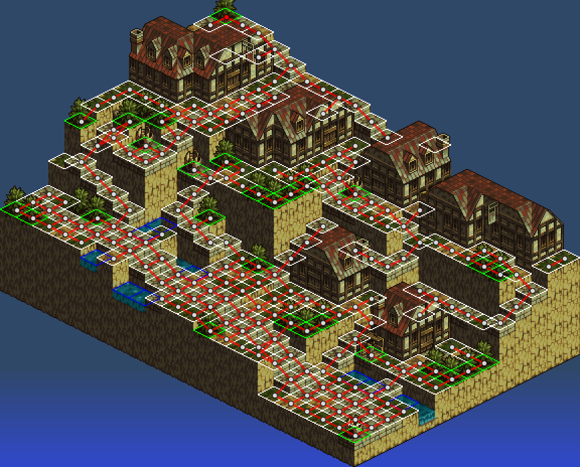
And the final extraction map can be depicted as follows:
gridArray = With[{allLayers =
     MapIndexed[With[{gridLocs = GridColorMap[#1, #2[[1]]  ]},
        Lookup[gridLocs, #, 0] & /@
         Table[{i, j}, {i, 1, 496}, {j, 1, 608}]] &,
      tileTypesLocs]},
   ReplaceAll[Table[Min[
      DeleteCases[
       allLayers[[All, i, j]], 0]],
     {i, 1, 496}, {j, 1, 608} ],
    \[Infinity] -> 0]
   ];


ImageAdd[ImageMultiply[im1,
  ArrayPlot[Sign[gridArray], PixelConstrained -> 1, Frame -> False]],
 ArrayPlot[gridArray, PixelConstrained -> 1, Frame -> False,
  ColorRules -> {0 -> Black, 1 -> White, 2 -> Green,
    3 -> Green, 4 -> Green, 5 -> Blue, 6 -> Red}]
 ]
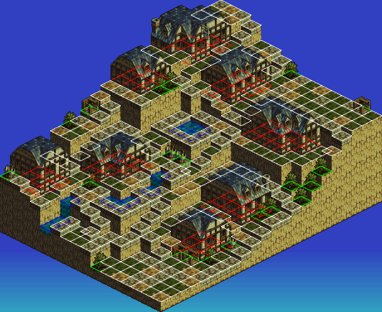
The tedious part is now done, and classifiers can be trained relatively easily:
positivesData = MapIndexed[Function[{set, num},
    # -> First[num] & /@ Catenate[KeyValueMap[
         Function[{key, vals},
          sortedImageGrids[key][[Sequence @@ #]] & /@ vals
          ], #] &@set]], tileTypesLocs];

allData = Union[Flatten[Values@sortedImageGrids]];

NegativeFrames[positives_] :=
 Map[# -> 0 &, Complement[allData, positives[[All, 1]]]]

AbsoluteTiming[
 binaryCFun =
   Classify[
    Join[positivesData[[1]], NegativeFrames[positivesData[[1]]]]];
 ]

AbsoluteTiming[
 detailedCFun = Classify[Join[Catenate[Most@positivesData],
     NegativeFrames[Catenate[Most@positivesData]]]];
 ]
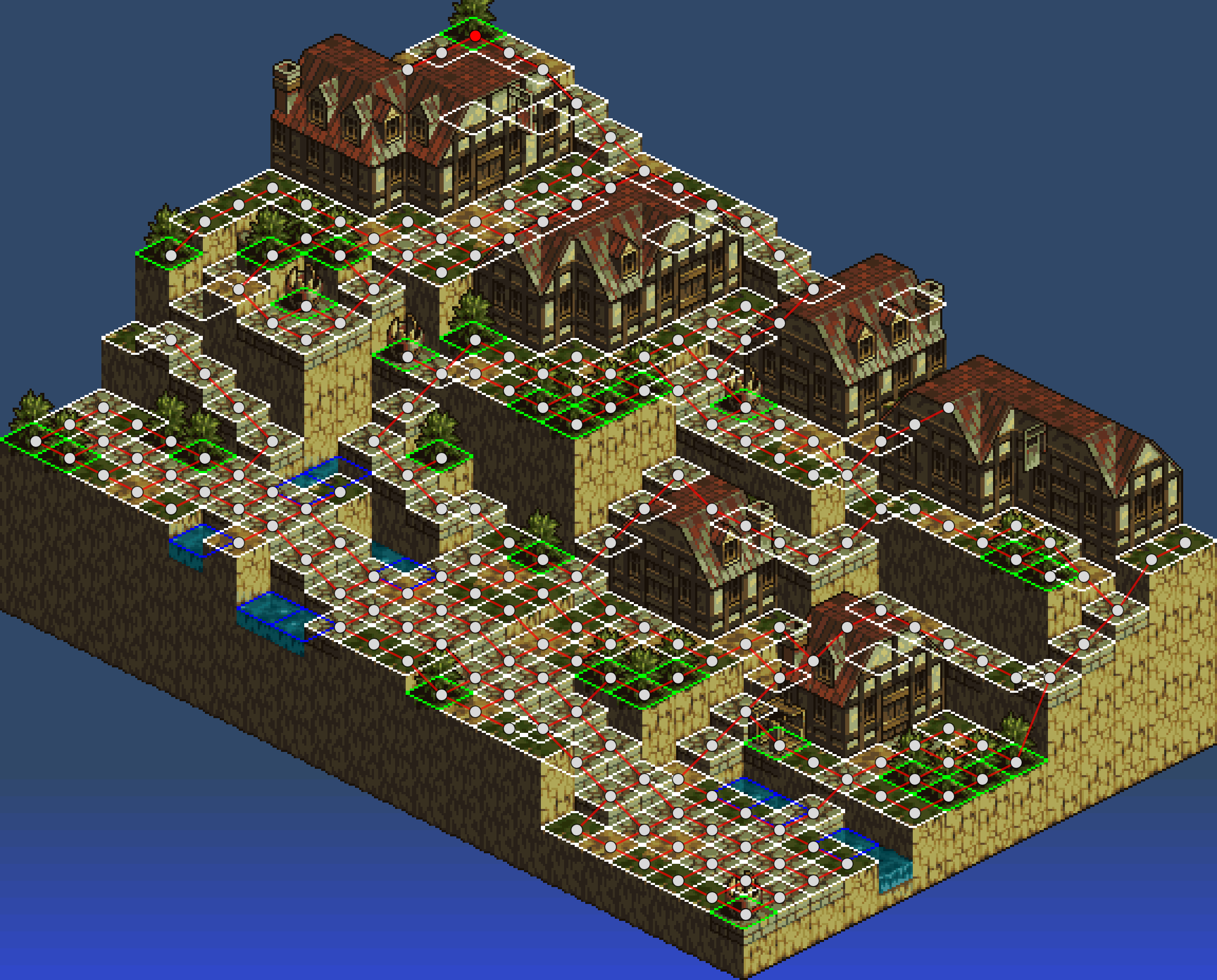
Skipping ahead by a few functions, here's what the classifier can do automatically after about 10 seconds of training and 10 seconds of analysis on another map from the same town:
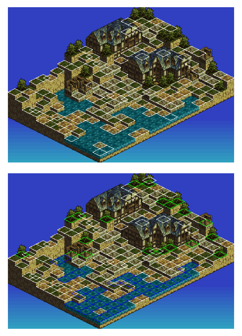
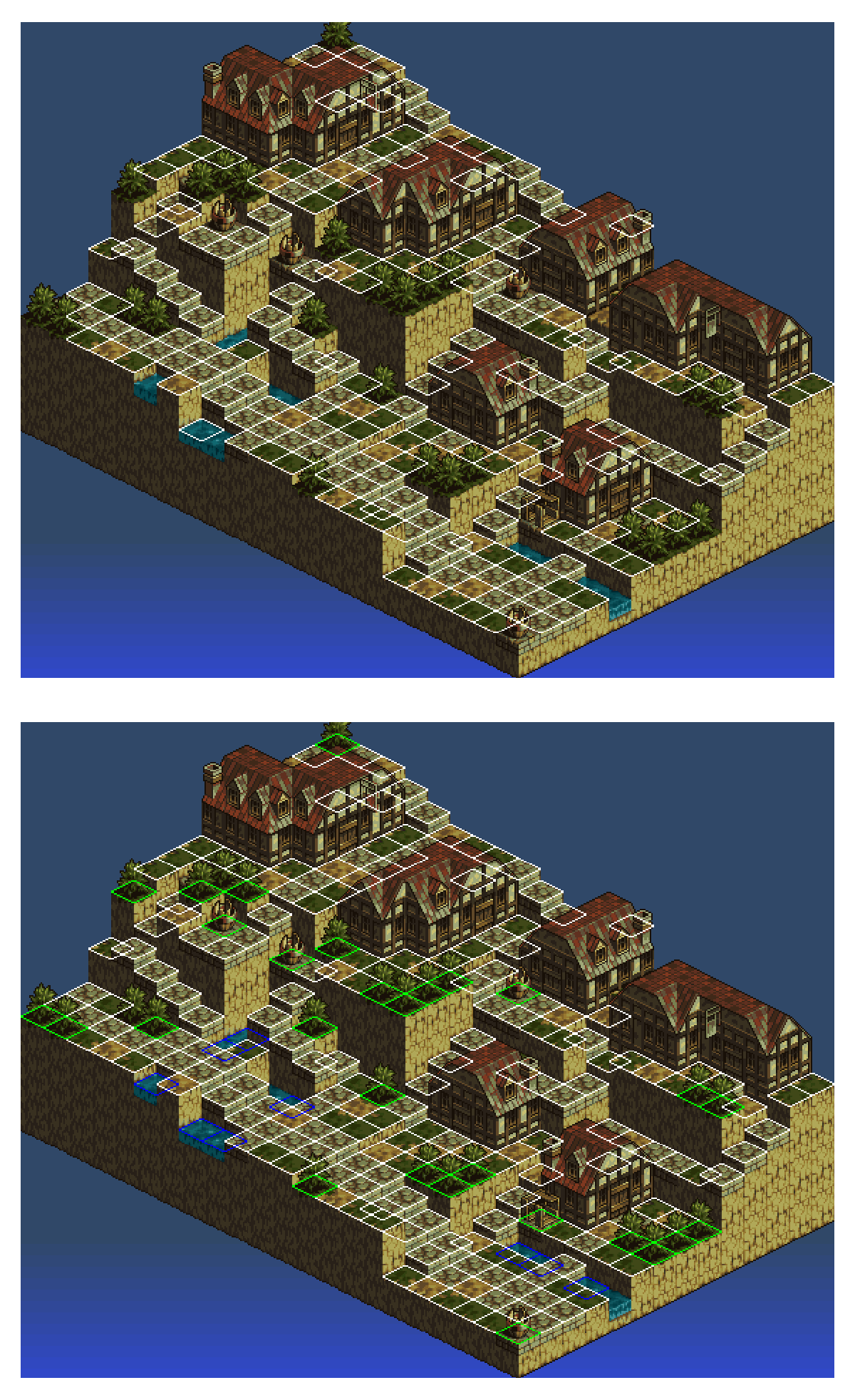
It's not perfect, but at least gets us to a decent starting place. For a more difficult test, we'll go to the next town over, where the roofs are red but the land is mostly the same (ha ha). The classifier still does pretty well:
imTest = ImageTake[ Import[
    "https://www.vgmaps.com/Atlas/SuperNES/TacticsOgre-LetUsClingTogether(J)-Rime-Chapter2-LawfulBattle(Unmarked).png"],
   {-464, -1}, {1, -1}];

dims = ImageDimensions@imTest
ImageDimensions[imTest]/{32, 16}
Out[]= {512, 352}
Out[]= {16, 22}

imageTestGrids = Association[MapThread[Rule, {
     Catenate[Outer[{#1 - 1, #2 - 1} &, {1, 2}, {1, 2}]],
     Catenate[Outer[ImagePartition[imTest, {32, 16}, {16, 8}
           ][[#1 ;; -1 ;; 2, #2 ;; -1 ;; 2]] &, {1, 2}, {1, 2}]
       ][[{3, 1, 2, 4}]]}]];

AbsoluteTiming[
 binaryTestData = Map[binaryCFun, imageTestGrids, {3}];
 ]

AbsoluteTiming[
 detailedTestData = Map[detailedCFun, imageTestGrids, {3}];
 ]

binaryGridData = With[{binaryGridLookup = Association[
      Map[# -> 1 &, Union[Flatten[KeyValueMap[
          DiamondOutline,
          Position[#, 1] & /@ binaryTestData
          ], 2]]]]},
   Lookup[binaryGridLookup, #, 0] & /@ Table[{i, j},
     {i, 1, dims[[2]]}, {j, 1, dims[[1]]}]];

detailedGridData = With[{detailedGridLookup = Association[
      Catenate[Function[{ind},
         Map[# -> ind &,
          Union[Flatten[KeyValueMap[
             DiamondOutline,
             Position[#, ind] & /@ detailedTestData
             ], 2]]]] /@ Range[6]]]},
   Lookup[detailedGridLookup, #, 0] & /@ Table[{i, j},
     {i, 1, dims[[2]]}, {j, 1, dims[[1]]}]];

processedIms = ImageAdd[ImageMultiply[imTest,
      ArrayPlot[Sign[#], PixelConstrained -> 1, Frame -> False]],
     ArrayPlot[#, PixelConstrained -> 1, Frame -> False,
      ColorRules -> {0 -> Black, 1 -> White, 2 -> Green,
        3 -> Green, 4 -> Green, 5 -> Blue, 6 -> Red}]
     ] & /@ {binaryGridData, detailedGridData};

ArrayPlot[Sign[gridArray], PixelConstrained -> 1, Frame -> False];

GraphicsColumn[Show[#, ImageSize -> 600] & /@ processedIms]
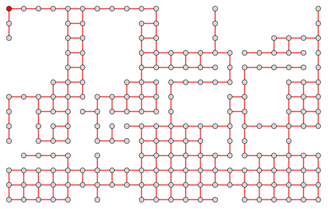
And taking the second graph in particular, we can extract a basic path graph:
detailedCentroids = Association[
   Catenate[Function[{ind},
      Map[# -> ind &,
       Union[Flatten[KeyValueMap[
          DiamondCentroid,
          Position[#, ind] & /@ detailedTestData
          ], 2]]]] /@ Range[6]]];

ExtractHeightGraph[data_, addVertices_List : {},
  deleteVertices_List : {},
  addEdges_List : {}, opts : OptionsPattern[Graph]
  ] := With[{g1 = EdgeAdd[NearestNeighborGraph[
      Complement[Union[Keys@Select[data, # < 5 &],
        addVertices], deleteVertices],
      {6, 24}], addEdges]},
  Graph[Select[EdgeList[g1],
    FreeQ[Subtract @@ #, 0] &
    ],
   opts,
   EdgeStyle -> Directive[Red, Thick], VertexSize -> 1/3,
   AspectRatio -> 1, VertexStyle -> {_ -> LightGray, {17, 225} -> Red},
   VertexCoordinates ->
    Map[# -> Reverse[{-1, 1} # + {464, 0} + {0, 0}] &, VertexList[g1]],
   VertexLabels -> Placed["Name", Tooltip]]]

Show[
 processedIms[[2]],
 graph0 = ExtractHeightGraph[detailedCentroids, VertexSize -> 2/3],
 PlotRange -> {{0, dims[[1]]}, {0, dims[[2]]}}, ImageSize -> dims
 ]
Again, this is pretty good analysis for only 10 seconds of work, but there are false positives as well as missing data points. At this point, we really should have a feedback loop where the initial path map is subsequently refined using non-local adjacency information. Working toward that, we allow arbitrary adding / deleting of vertices and edges to obtain the following:
Show[
 processedIms[[2]],
 nnGraph = ExtractHeightGraph[detailedCentroids,
   {{89, 289}, {113, 145}, {153, 369}, {177, 257}, {185, 273}, {193,
     449},
    {201, 433}, {241, 337}, {297, 401}, {313, 385}, {353, 433}, {361,
     449},
    {209, 81}, {33, 193}},
   {{57, 257}, {113, 321}, {129, 113}, {145, 97}, {313, 417}, {353,
     257}},
   {UndirectedEdge[{361, 481}, {321, 497}],
    UndirectedEdge[{289, 529}, {265, 545}]}
   ],
 PlotRange -> {{0, dims[[1]]}, {0, dims[[2]]}}, ImageSize -> 2 dims
 ]
In addition to correcting False positives / negatives, we have also added edges in the last column to connect disconnected components. This graph is sufficiently well-drawn in two dimensions that we can traverse vertices while extracting height information:
Pixelto3D = Association[Join[{
     {-16, -8} -> {0, 1, 0},
     {16, -8} -> {1, 0, 0},
     {16, 8} -> {0, -1, 0},
     {-16, 8} -> {-1, 0, 0},

     {-16, -16} -> {0, 1, -1},
     {16, -16} -> {1, 0, -1},
     {16, 16} -> {0, -1, 1},
     {-16, 16} -> {-1, 0, 1}
     }, {
     (* semi-hacked values *)
     {-16, 40} -> {-1, 0, 4},
     {-16, 24} -> {-1, 0, 2},
     {16, -40} -> {1, 0, -4},
     {16, -24} -> {1, 0, -2}
     }
    ]];

IterateAll[nnGraph_][inits_] :=
 With[{newVertices = Catenate[IterateVertex[nnGraph] /@ First[inits]]},
  {Complement[newVertices, Last[inits]], Union[
    newVertices,
    Last[inits]]}
  ]

IterateVertex[nnGraph_][coords_Rule] := With[
    {check = Lookup[Pixelto3D, Key[Reverse[First[coords] - #]], True]},
    If[TrueQ[check], Nothing,
     # -> Plus[Last[coords], check]
     ]] & /@ VertexOutComponent[nnGraph, First@coords, {1}]

heightPathMap = Last[NestWhile[IterateAll[nnGraph],
    Table[{{17, 225} -> {1, 1, -1}}, 2],
    UnsameQ[First[#], {}] &]];
g2 = Graph[Subgraph[nnGraph, First /@ heightPathMap],
  VertexCoordinates ->
   Map[First[#] -> Times[Last[#][[{2, 1}]], {1, -1}] &, %],
  PlotRange -> All]
Most of the missing vertices correspond to location of buildings or water, which could potentially be filled in automatically (but this would require more work on classifier functions and feedback loops). Vertices of the graph are encoded with information to project most of the terrain into 3D voxels:
With[{heightMap = Normal@SparseArray[
     Last[#][[1 ;; 2]] -> (Last[#][[3]] + 22) & /@ heightPathMap]},
 Graphics3D[{
   MapIndexed[{
      Lighter[Brown, 0.6],
      Cuboid[Append[#2, 0], Append[#2 + {1, 1}, #1/2]]} &,
    heightMap, {2}]},
  ViewPoint -> {Infinity, Infinity, Infinity},
  ViewVertical -> {0, 0, 1}, Boxed -> False]]
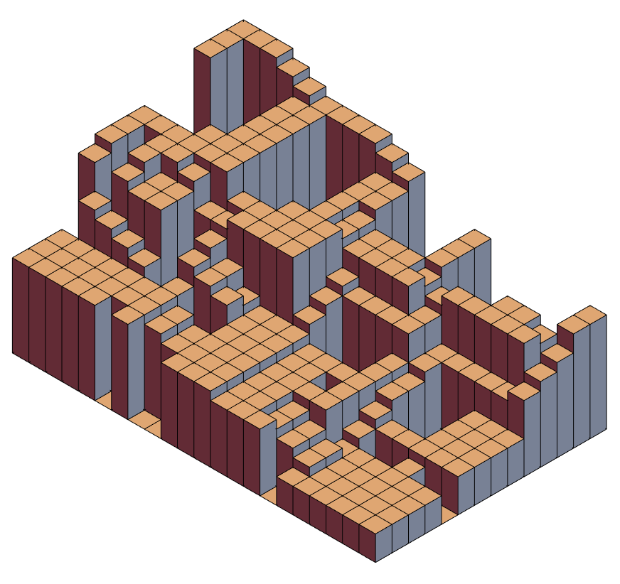
As far as proof of concept goes, we can declare victory. However if we want a perfect classifier that doesn't need any human intervention, obviously we would need to revise the basic algorithm to make use of a self-consistent loop including global structure information.
To return to what the Kotaku reviewer said (which seems to be a common criticism of the remaster):
I don’t know how feasible it would have been to try and give Reborn the Octopath Traveler or Triangle Strategy HD-2D pixel art look, but I wish the game felt as beautiful to look at as it is to play and listen to...
Game developers would likely have access to more primitive data including height maps and tile sets, but it would still take a considerable effort to redraw all assets as 3D voxel plots. Such effort might not contribute to a significant game play improvement because most of maps are designed with a uni-directional height gradient assuming a fixed camera location (Ex: All maps above). It would probably be better to just save the money for a sequel, with an entirely new set of maps designed with multiple viewpoints in mind. Or perhaps a sequel will feature the first completely-connected, fully-explorable "open world" geometry (too much to ask for?).
While it may be difficult to classify map data and transform it into three-dimensions, we can at least make some decent progress in a few days. An even more difficult set of issues has to do with balancing character interaction and giving computer controlled NPCs realistic decision making. This question could also potentially be approached via machine learning, but not so easily. Perhaps for another day...


