The MRB constant record computations are given here in the Wolfram community. To help in the loading times of that extensive discussion, I've moved its applications to this separate discussion.
CMRB and its applications
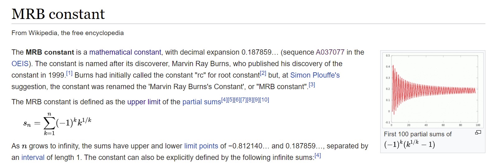
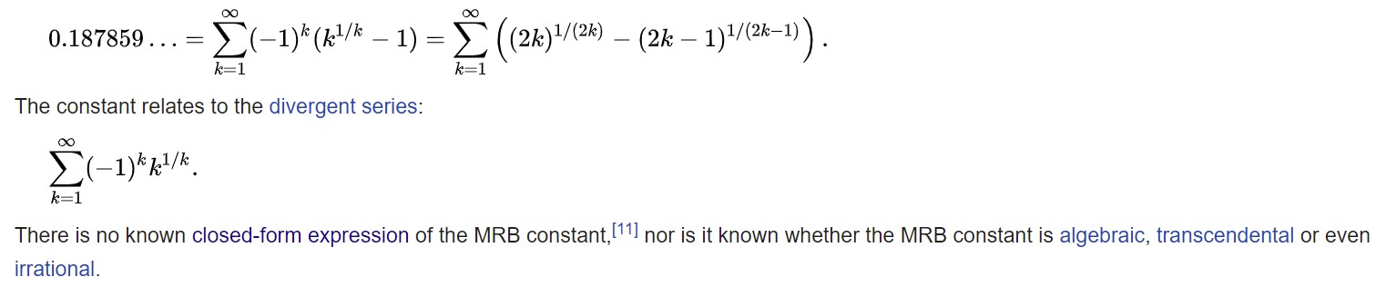
Definition 1 CMRB is defined at https://en.wikipedia.org/wiki/MRB_constant .
From Wikipedia:
References
 Plouffe, Simon. "mrburns". Retrieved 12 January 2015.
 Burns, Marvin R. (23 January 1999). "RC". math2.org. Retrieved 5 May 2009.
 Plouffe, Simon (20 November 1999). "Tables of Constants" (PDF). Laboratoire de combinatoire et d'informatique mathématique. Retrieved 5 May 2009.
 Weisstein, Eric W. "MRB Constant". MathWorld.
 Mathar, Richard J. (2009). "Numerical Evaluation of the Oscillatory Integral Over exp(iπx) x^*1/x) Between 1 and Infinity". arXiv:0912.3844 [math.CA].
 Crandall, Richard. "Unified algorithms for polylogarithm, L-series, and zeta variants" (PDF). PSI Press. Archived from the original (PDF) on April 30, 2013. Retrieved 16 January 2015.
 (sequence A037077 in the OEIS)
 (sequence A160755 in the OEIS)
 (sequence A173273 in the OEIS)
 Fiorentini, Mauro. "MRB (costante)". bitman.name (in Italian). Retrieved 14 January 2015.
 Finch, Steven R. (2003). Mathematical Constants. Cambridge, England: Cambridge University Press. p. 450. ISBN 0-521-81805-2.
`
The following equation that was shown in the Wikipedia definition shows how closely the MRB constant is related to root two.
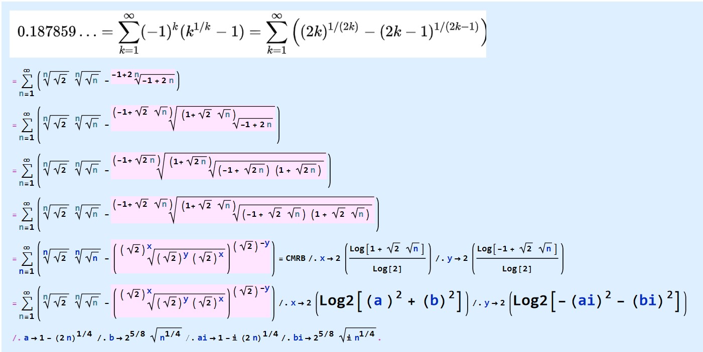
In[1]:= N[Sum[Sqrt[2]^(1/n)* Sqrt[n]^(1/n) - ((Sqrt[2]^y*Sqrt[2]^x)^(1/Sqrt[2]^x))^Sqrt[2]^(-y)/.
x -> 2*Log2[a^2 + b^2] /.
y -> 2*Log2[-ai^2 - bi^2] /.
a -> 1 - (2*n)^(1/4) /.
b -> 2^(5/8)*Sqrt[n^(1/4)] /.
ai -> 1 - I*(2*n)^(1/4) /.
bi -> 2^(5/8)*Sqrt[I*n^(1/4)], {n, 1, Infinity}], 7]

Out[1]= 0.1878596 + 0.*10^-8 I
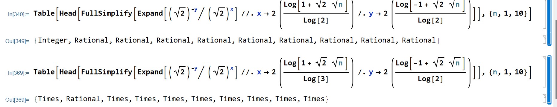
The complex roots and powers above are found to be well-defined because we get all either "integer" and "rational" the first of the following lists only, also by working from the bottom to the top of the above list of equations.
Code:
In[349]:= Table[
 Head[FullSimplify[
   Expand[(Sqrt[2])^-y/(Sqrt[2])^x] //.
     x -> 2 (Log[1 + Sqrt[2] Sqrt[n]]/Log[2]) /.
    y -> 2 (Log[-1 + Sqrt[2] Sqrt[n]]/Log[2])]], {n, 1, 10}]

Out[349]= {Integer, Rational, Rational, Rational, Rational, Rational, \
Rational, Rational, Rational, Rational}

In[369]:= Table[
 Head[FullSimplify[
   Expand[(Sqrt[2])^-y/(Sqrt[2])^x] //.
     x -> 2 (Log[1 + Sqrt[2] Sqrt[n]]/Log[3]) /.
    y -> 2 (Log[-1 + Sqrt[2] Sqrt[n]]/Log[2])]], {n, 1, 10}]

Out[369]= {Times, Rational, Times, Times, Times, Times, Times, Times, \
Times, Times}
Definition 2 CMRB is defined at http://mathworld.wolfram.com/MRBConstant.html.
From MathWorld:
SEE ALSO:
Glaisher-Kinkelin Constant, Power Tower, Steiner's Problem
REFERENCES:
Burns, M. R. "An Alternating Series Involving n^(th) Roots." Unpublished note, 1999.

Burns, M. R. "Try to Beat These MRB Constant Records!" http://community.wolfram.com/groups/-/m/t/366628.

Crandall, R. E. "Unified Algorithms for Polylogarithm, L-Series, and Zeta Variants." 2012a.
http://www.marvinrayburns.com/UniversalTOC25.pdf.
Crandall, R. E. "The MRB Constant." §7.5 in Algorithmic Reflections: Selected Works. PSI Press, pp. 28-29, 2012b.

Finch, S. R. Mathematical Constants. Cambridge, England: Cambridge University Press, p. 450, 2003.

Plouffe, S. "MRB Constant." http://pi.lacim.uqam.ca/piDATA/mrburns.txt.

Sloane, N. J. A. Sequences A037077 in "The On-Line Encyclopedia of Integer Sequences."

Referenced on Wolfram|Alpha: MRB Constant
CITE THIS AS:
Weisstein, Eric W. "MRB Constant." From MathWorld--A Wolfram Web Resource. https://mathworld.wolfram.com/MRBConstant.html
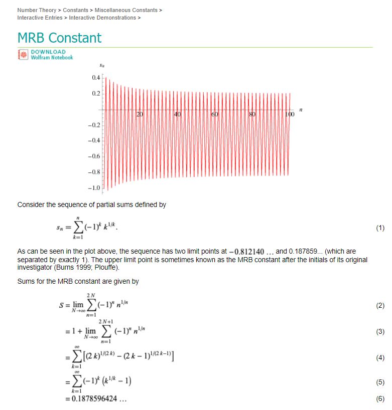
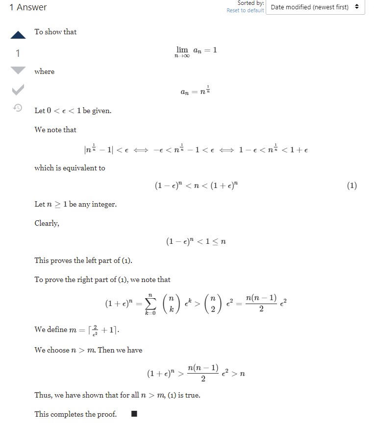
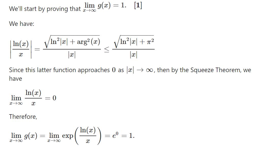
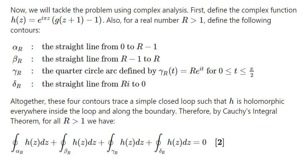
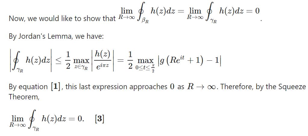
How would we show that any of the series in the above MathWorld definition are convergent, or even absolutely convergent?
For "a"k=k1/k, given that the sequence is monotonically decreasing according to Steiner's Problem, next, we would like to show (5) is the alternating sum of a sequence that converges to 0 monotonically and use the Alternating series test to see that it is conditionally convergent
Here is proof that 1 is the limit of "a" as k goes to infinity:
Here are many other proofs that 1 is the limit of "a" as k goes to infinity.
Thus, (k1/k-1) is a monotonically decreasing and bounded below by 0 sequence.
If we want an absolutely convergent series, we can use (4).
Sk which, since the sum of the absolute values of the summands is finite, the sum converges absolutely!
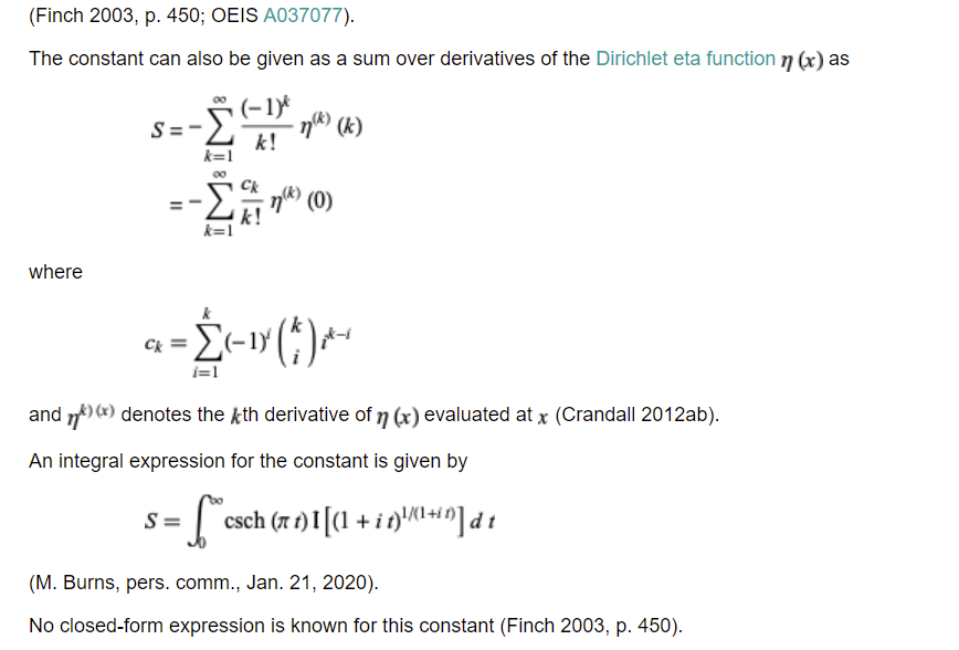
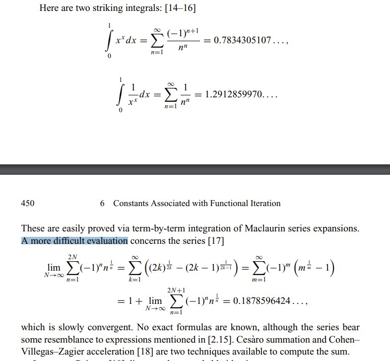
There is no closed-form for CMRB in the MathWorld definition; this could be due to the following: in Mathematical Constants,( Finch, S. R. Mathematical Constants, Cambridge, England: Cambridge University Press, p. 450), Steven Finch wrote that it is difficult to find an "exact formula" (closed-form solution) for it.
Real-World, and beyond, Applications
CMRB as a Growth Model
Its factor  models the interest rate to multiply an investment k times in k periods, as well as "other growth and decay functions involving the more general expression
  , as in Plot 1A," because
r=(k^(1/k)-1);Animate[ListPlot[l=Accumulate[Table[(r+1)^n,{k,100}]], PlotStyle->Red,PlotRange->{0,150},PlotLegends->{"\!\(\*UnderscriptBox[\(\[Sum]\), \(\)]\)(r+1\!\(\*SuperscriptBox[\()\), \(n\)]\)/.r->(\!\(\*SuperscriptBox[\(k\), \(1/k\)]\)-1)/.n->"n},AxesOrigin->{0,0}],{n,0,5}]
Plot 1A 
The discrete rates looks like the following.
r = (k^(1/k) - 1); me =
 Animate[ListPlot[l = Table[(r + 1)^n, {k, 100}], PlotStyle -> Red,
   PlotLegends -> {"(r+1)^n/.r->\!\(\*SuperscriptBox[\(k\), \
\(1/k\)]\)=1/.n->", n}, AxesOrigin -> {0, 0},
   PlotRange -> {0, 7}], {n, 1, 5}]
That factor models not only discretely compounded rates but continuous too, ie 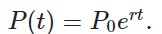
By entering
Solve[P*E^(r*t) == P*(t^(1/t) - 1), r]
we see, for 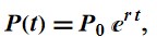
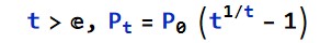
gives an effect of continuous decay of 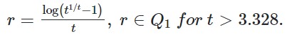 Here Q1 means the first Quarter form 0 to -1.
The alternating sum of the principal of those continuous rates, i.e. P=(-1)t er t is the MRB constant (CMRB): 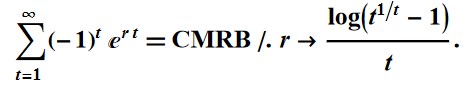
In[647]:= NSum[(-1)^t ( E^(r*t)) /. r -> Log[-1 + t^(1/t)]/t, {t, 1,
  Infinity}, Method -> "AlternatingSigns", WorkingPrecision -> 30]

Out[647]= 0.18785964246206712024857897184
Its integral (MKB) is an analog to CMRB : 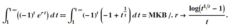
In[1]:= NIntegrate[(-1)^t (E^(r*t)) /. r -> Log[-1 + t^(1/t)]/t, {t,
1, Infinity I}, Method -> "Trapezoidal", WorkingPrecision -> 30] -
2 I/Pi

   Out[1]= 0.0707760393115288035395280218303 -
    0.6840003894379321291827444599927 I
So, integrating P yields about 1/2 greater of a total than summing:
In[663]:=
CMRB = NSum[(-1)^n ( Power[n, ( n)^-1] - 1), {n, 1, Infinity},
   Method -> "AlternatingSigns", WorkingPrecision -> 30];

 In[664]:=
MKB = Abs[
   NIntegrate[(-1)^t ( E^(r*t)) /. r -> Log[-1 + t^(1/t)]/t, {t, 1,
      Infinity I}, Method -> "Trapezoidal", WorkingPrecision -> 30] -
    2 I/Pi];

In[667]:= MKB - CMRB

Out[667]= 0.49979272646562724956073343752
Next:
CMRB from Geometric Series and Power Series
The MRB constant: 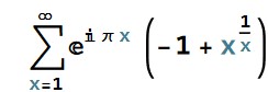 is closely related to geometric series:
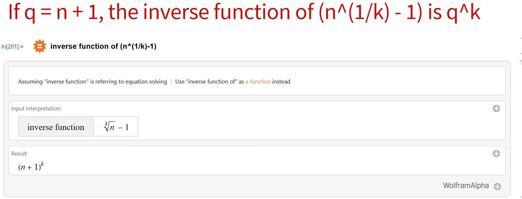
The inverse function of the "term" of the MRB constant, i.e. x^(1/x) within a certain domain is solved for in this link,
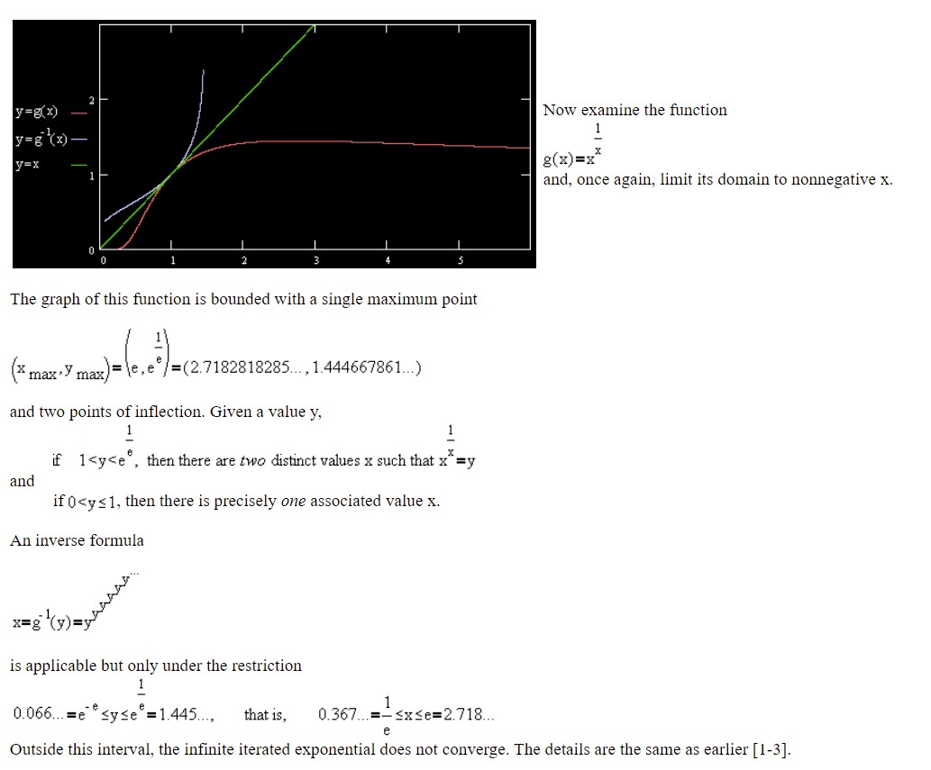
...
Now we have the following for the orientated area, from 0 to 1, between the graph of that term and the axis.
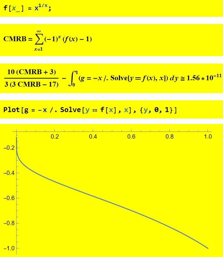
In[344]:= f[x_] = x^(1/x);

In[346]:= CMRB =
 NSum[(-1)^x (f[x] - 1), {x, 1, Infinity}, WorkingPrecision -> 20]

Out[346]= 0.18785964246207

In[350]:= (10 (CMRB + 3))/(3 (3 CMRB - 17)) -
 NIntegrate[g = -x /. Solve[y == f[x], x], {y, 0, 1},
  WorkingPrecision -> 20]

Out[350]= {1.5605*10^-11}
Consider the following about a slight generalization of that term.
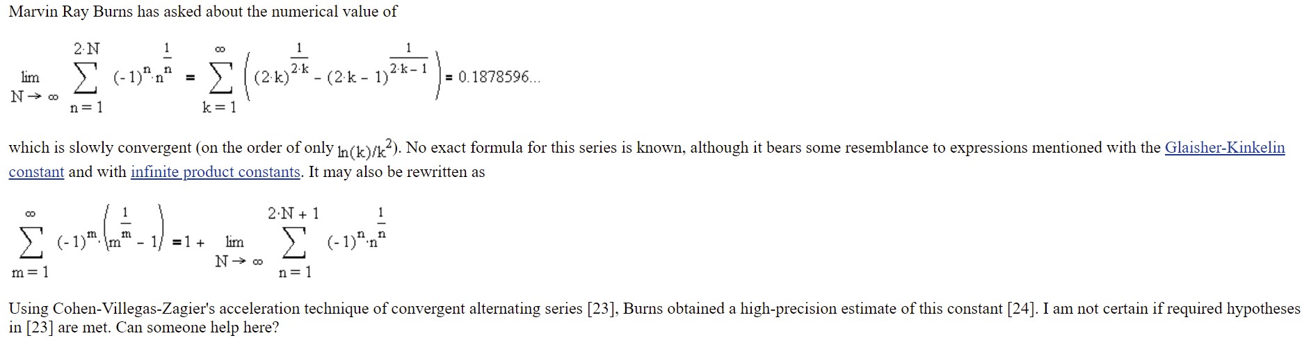
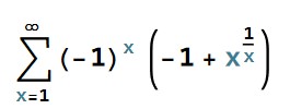
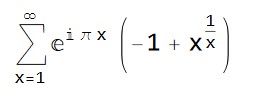
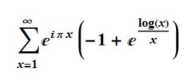
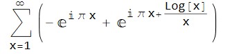
CMRB can be written in geometric series form:
CMRB= 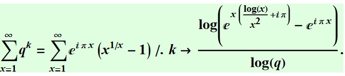
In[240]:= N[Quiet[(Sum[q^k, {x, 1, Infinity}] /.
          k -> Log[-E^(I*Pi*x) + E^(x*(I*Pi + Log[x]/x^2))]/Log[q]) -
       Sum[E^(I*Pi*x)*(-1 + x^(1/x)), {x, 1, Infinity}]]]

Out[240]= -4.163336342344337*^-16
Why would we express CMRB so? I'm not entirely sure, but we do have the following interestingly intricate graphs that go towards the value of the MRB constant and the MRB constant-1 as the input gets large. 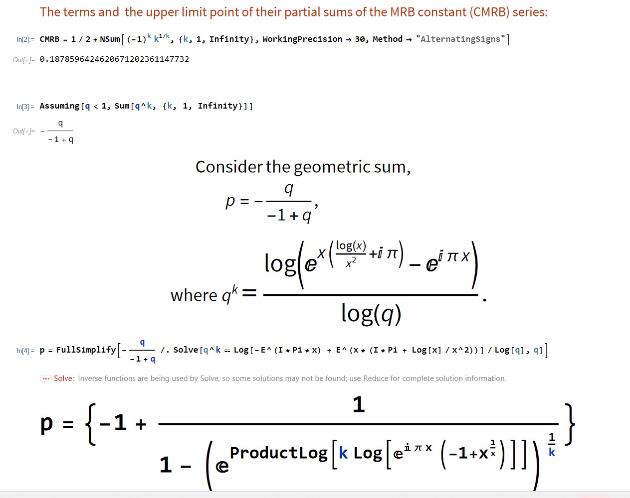
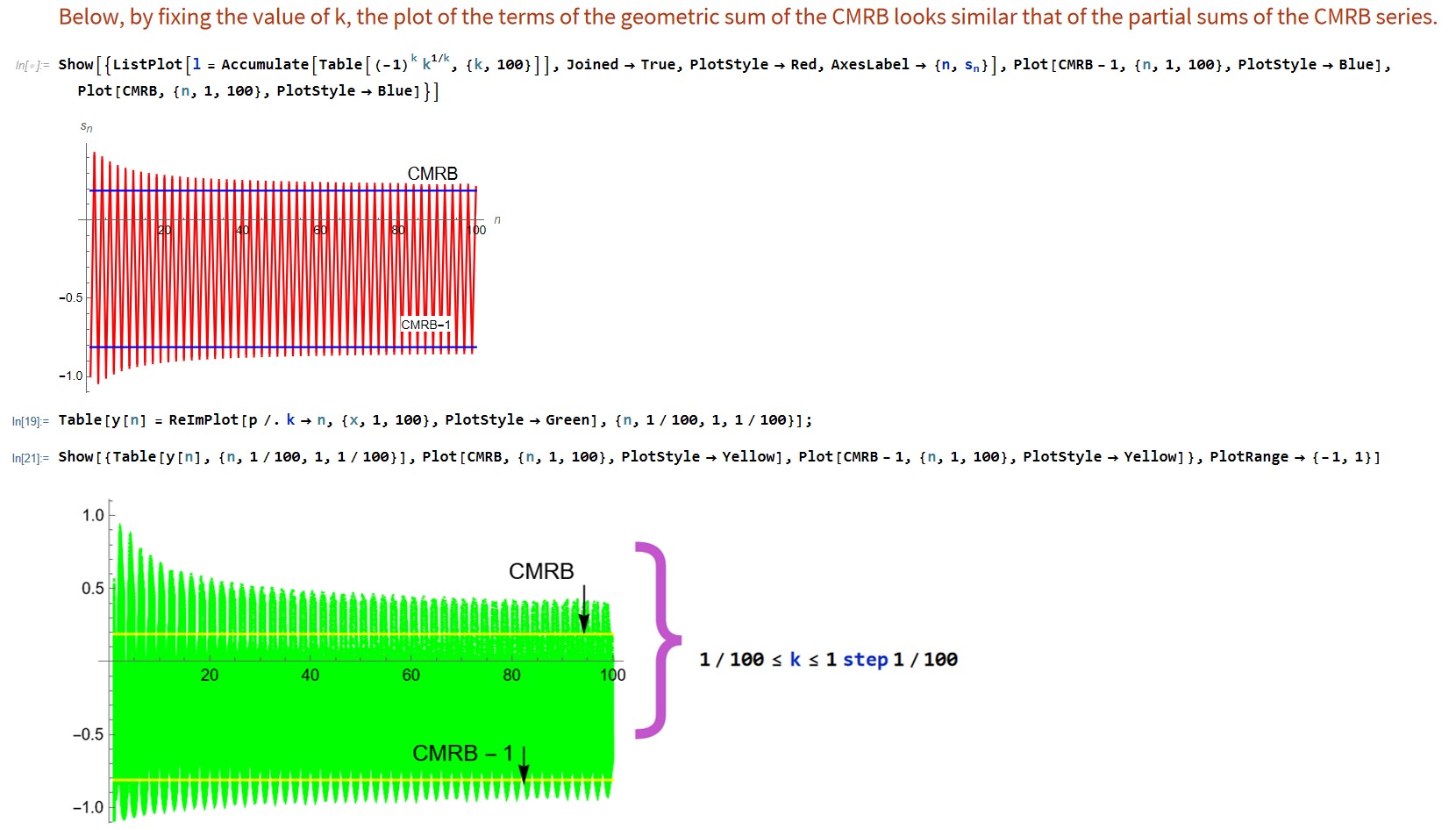
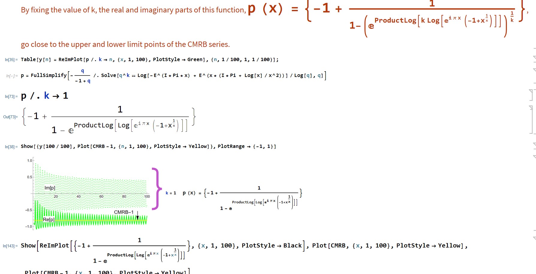
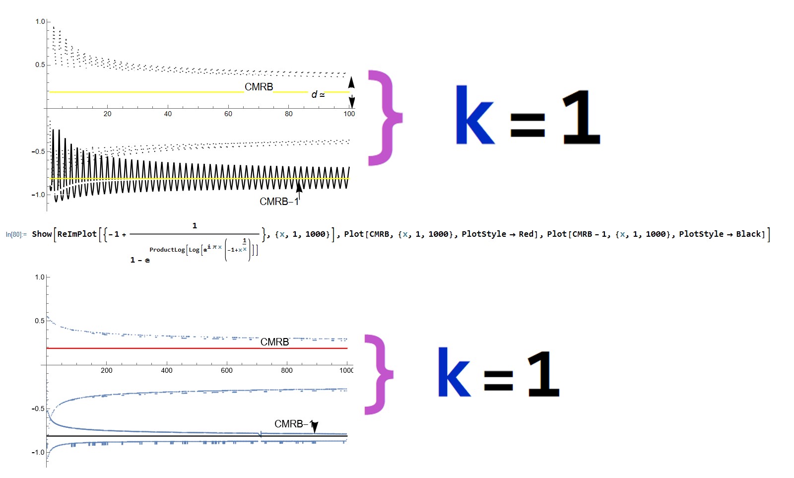
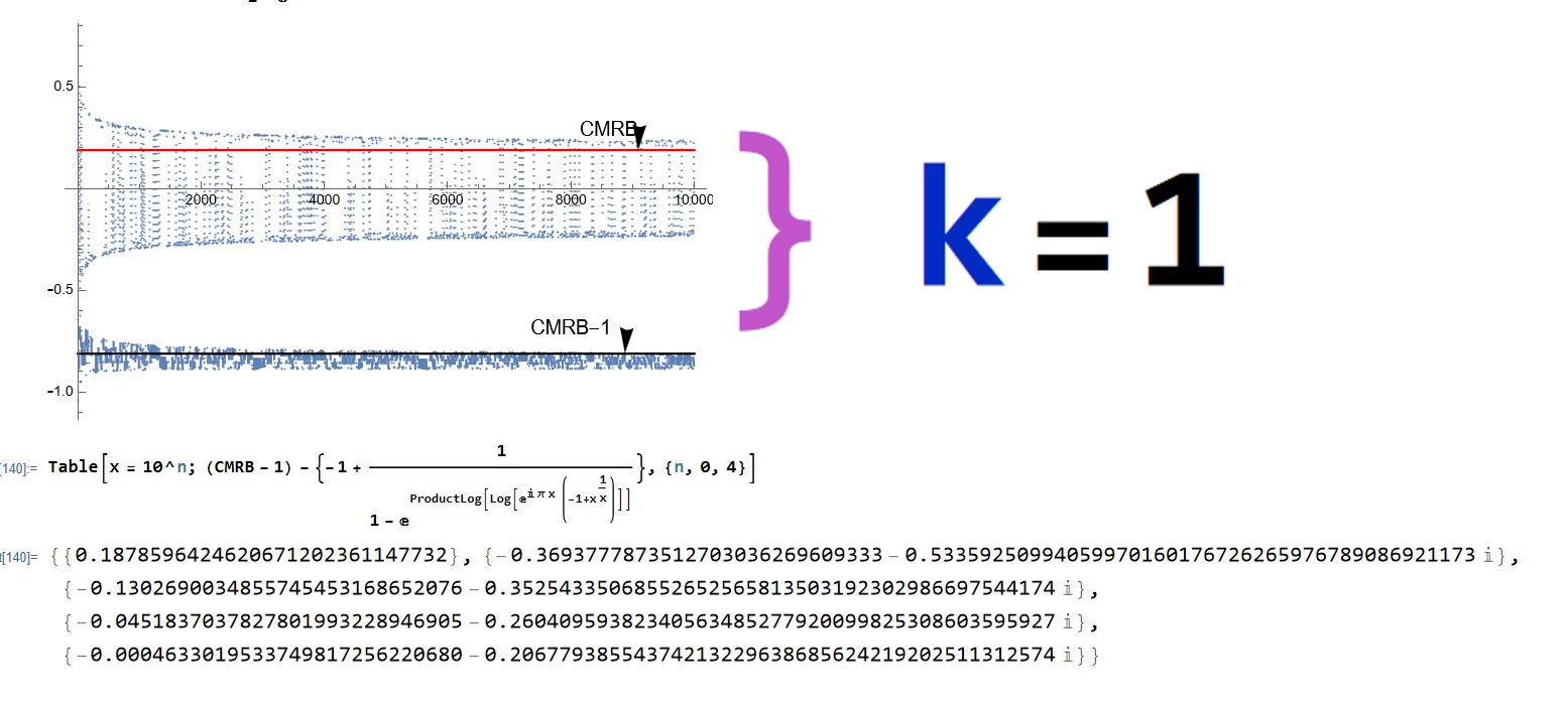
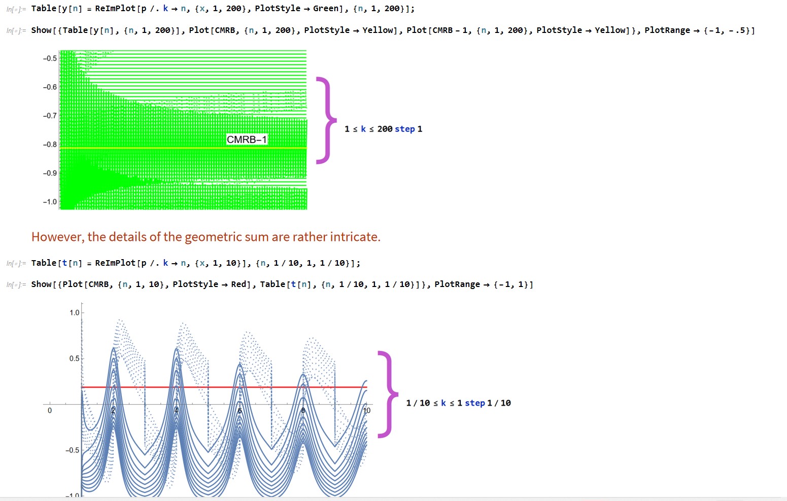
see notebook here.
Next
The Geometry of the MRB constant
In 1837 Pierre Wantzel proved that an nth root of a given length cannot be constructed if n is not a power of 2 (as mentioned here in Wikipedia). However, the following is a little different.
For  on November 21, 2010, I coined a multiversal analog to, Minkowski space that plots their values from constructions arising from a peculiar non-euclidean geometry, below, and fully in this vixra draft.
As in Diagram 2, we give each n-cube a hyperbolic volume (content) equal to its dimension,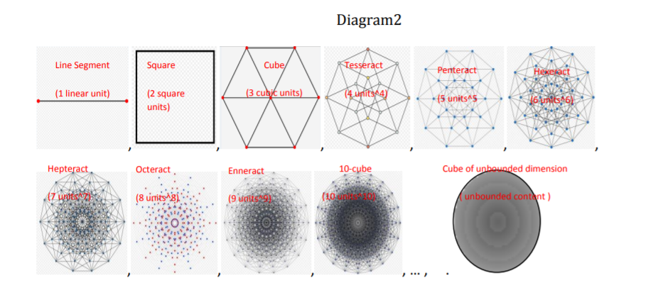 Geometrically, as in Diagram3, on the y,z-plane line up an edge of each n-cube. The numeric values displayed in the diagram are the partial sums of S[x_] =
 Sum[(-1)^n*n^(1/n), {n, 1, 2*u}] where u is an positive integer. Then M is the MRB constant.
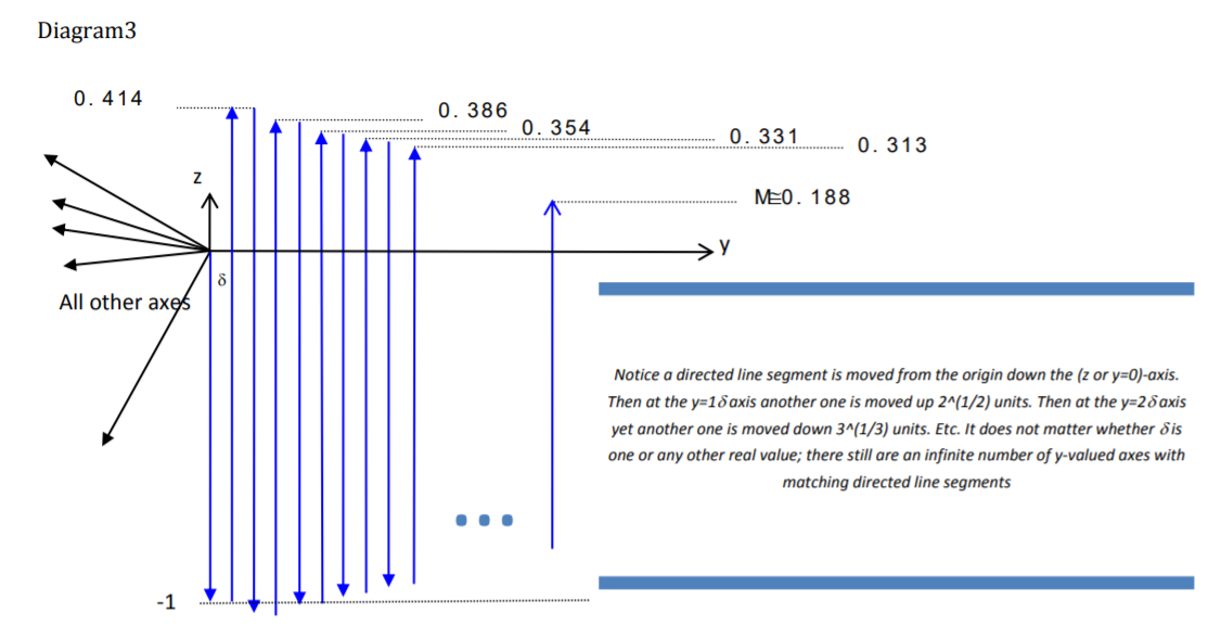
Join[ Table[N[S[x]], {u, 1, 4}], {"..."}, {NSum[(-1)^n*(n^(1/n) - 1), {n, 1, Infinity}]}]
Out[421]= {0.414214, 0.386178, 0.354454, 0.330824, "...", 0.18786}
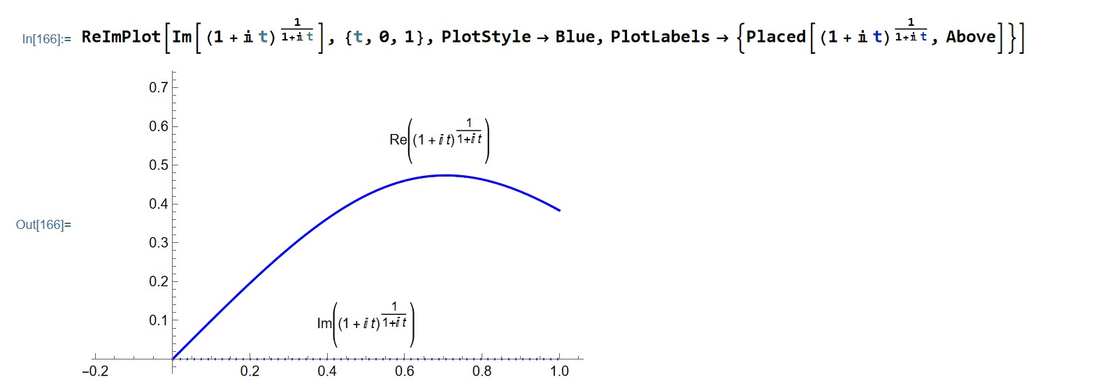
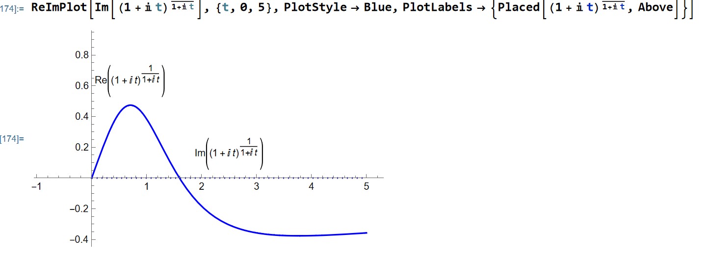
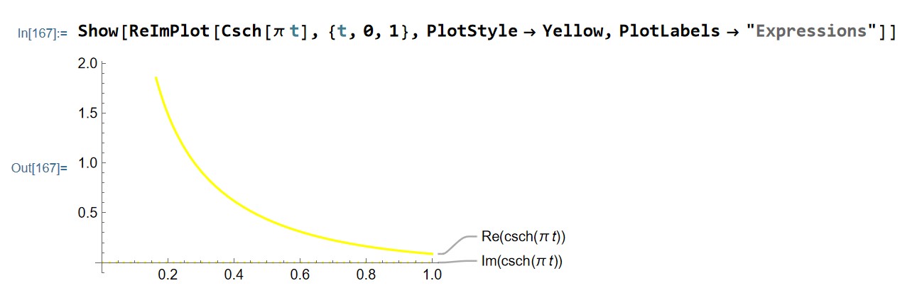
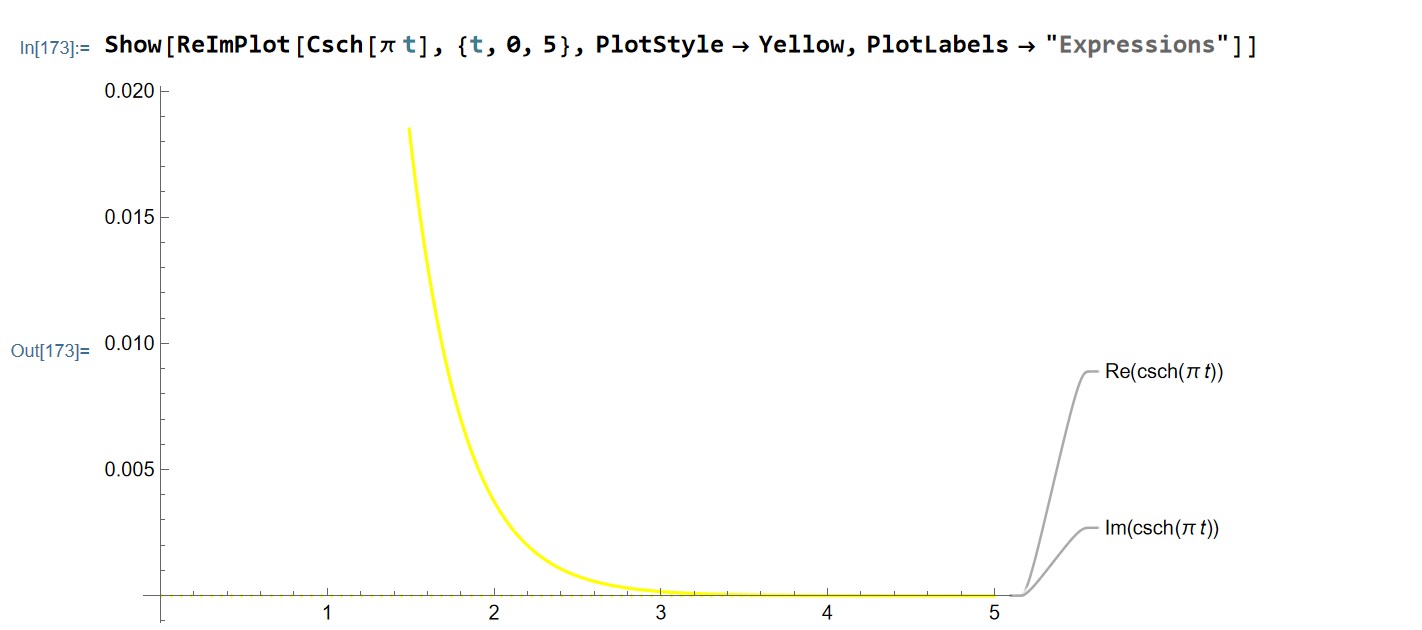
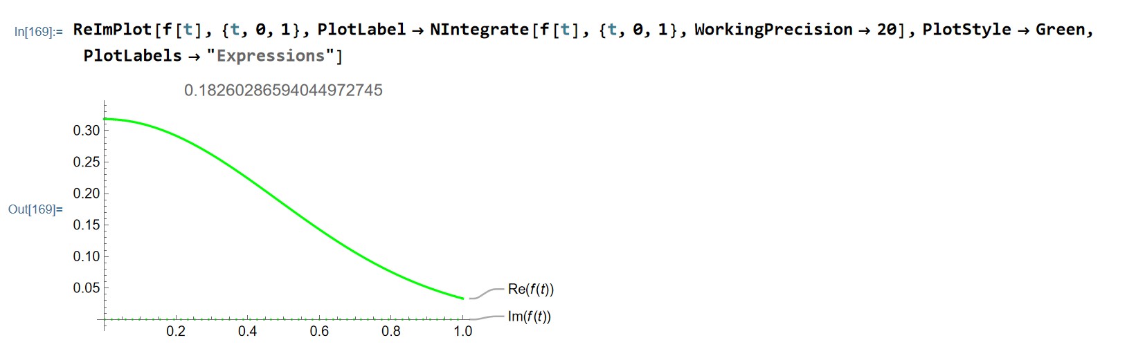
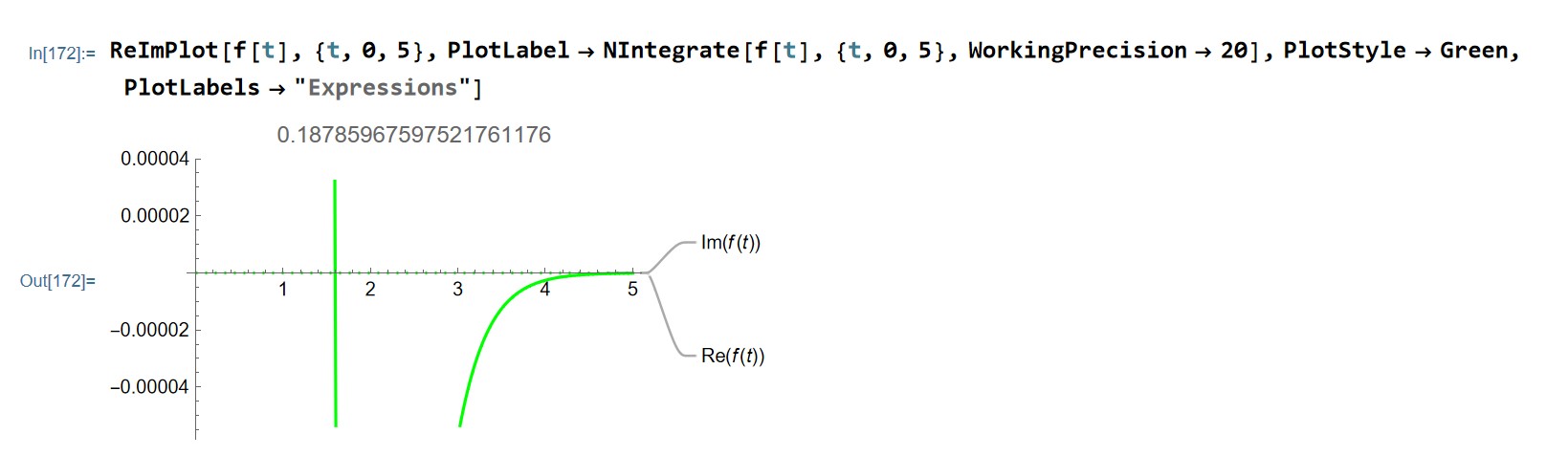
Here are views of some regions of the plot of a definite integral equal to CMRB..
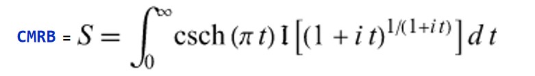
In[66]:= Csch[Pi t] Im[(1 + I t)^(1/(1 + I t))]
Out[66]= Csch[[Pi] t] Im[(1 + I t)^(1/(1 + I t))]
In[67]:= f[t_] = Csch[Pi t] Im[(1 + I t)^(1/(1 + I t))]
Out[67]= Csch[[Pi] t] Im[(1 + I t)^(1/(1 + I t))]
ReImPlot[Im[(1 + I t)^(1/(1 + I t))], {t, 0, 1}, PlotStyle -> Blue,
 PlotLabels -> {Placed[(1 + I t)^(1/(1 + I t)), Above]}]
ReImPlot[Im[(1 + I t)^(1/(1 + I t))], {t, 0, 5}, PlotStyle -> Blue,
 PlotLabels -> {Placed[(1 + I t)^(1/(1 + I t)), Above]}]
Show[ReImPlot[Csch[\[Pi] t], {t, 0, 1}, PlotStyle -> Yellow,
  PlotLabels -> "Expressions"]]
Show[ReImPlot[Csch[\[Pi] t], {t, 0, 5}, PlotStyle -> Yellow,
  PlotLabels -> "Expressions"]]
ReImPlot[f[t], {t, 0, 1},
 PlotLabel -> NIntegrate[f[t], {t, 0, 1}, WorkingPrecision -> 20],
 PlotStyle -> Green, PlotLabels -> "Expressions"]
ReImPlot[f[t], {t, 0, 5},
 PlotLabel -> NIntegrate[f[t], {t, 0, 5}, WorkingPrecision -> 20],
 PlotStyle -> Green, PlotLabels -> "Expressions"]
Next
MeijerG Representation
From its integrated analog, I found a MeijerG representation for CMRB.
The search for it began with the following:
On 10/10/2021, I found the following proper definite integral that leads to almost identical proper integrals from 0 to 1 for CMRB and its integrated analog.
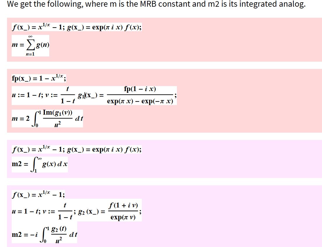
See notebook in this link.
Here is a MeijerG function for the integrated analog. See (proof) of discovery.
f(n)=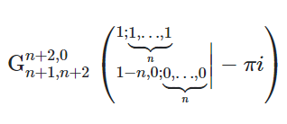 .
.
`
In[135]:=f[n_]:=MeijerG[{{},Table[1,{n+1}]},{Prepend[Table[0,n+1],-n+1],{}},-\[ImaginaryI]\[Pi]];`
In[337]:=M2=NIntegrate[E^(I Pi x)(SuperscriptBox["x", FractionBox["1", "x"]]-1),
{x,1,Infinity I},WorkingPrecision->100]
Out[337]=0.07077603931152880353952802183028200136575469620336302758317278816361845726438203658083188126617723821-0.04738061707035078610720940650260367857315289969317363933196100090256586758807049779050462314770913485 \[ImaginaryI]
I wonder if there is one for the MRB constant sum (CMRB)?
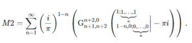
According to "Primary Proof 1" and "Primary Proof 3" shown below along with the section prefixed by the phrase "So far I came up with," it can be proven that for G being the Wolfram MeijerG function
and f(n)=, and 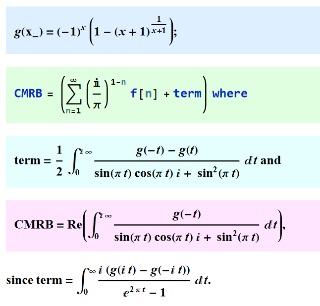
g[x_] = (-1)^x (1 - (x + 1)^(1/(x + 1)));

In[52]:= (1/2)*
 NIntegrate[(g[-t] - g[t])/(Sin[Pi*t]*Cos[Pi*t]*I + Sin[Pi*t]^2), {t,
   0, I*Infinity}, WorkingPrecision -> 100,
     Method -> "GlobalAdaptive"]

Out[52]= 0.\
1170836031505383167089899122239912286901483986967757585888318959258587\
7430027817712246477316693025869 +
 0.0473806170703507861072094065026036785731528996931736393319610009025\
6586758807049779050462314770913485 I


In[57]:= Re[
 NIntegrate[
  g[-t]/(Sin[Pi*t]*Cos[Pi*t]*I + Sin[Pi*t]^2), {t, 0, I*Infinity},
  WorkingPrecision -> 100,
     Method -> "GlobalAdaptive"]]

Out[57]= 0.\
1878596424620671202485179340542732300559030949001387861720046840894772\
315646602137032966544331074969
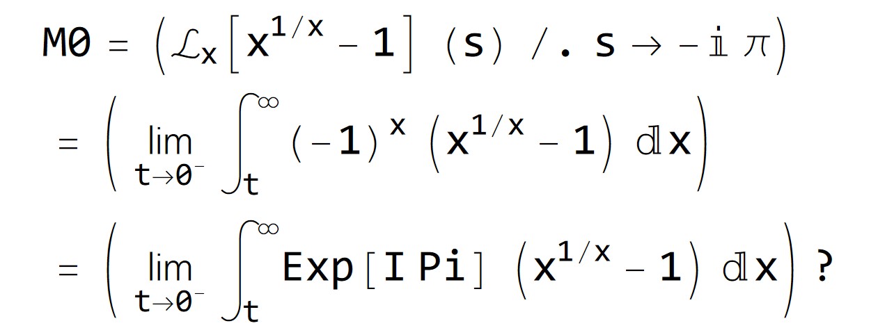
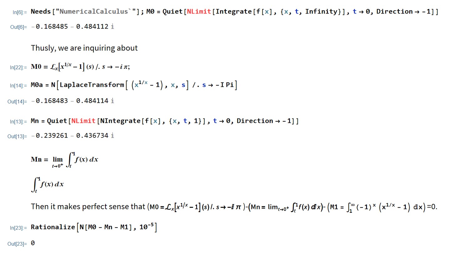
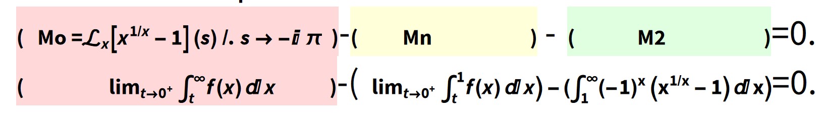
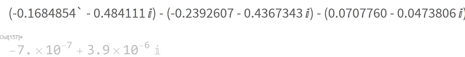
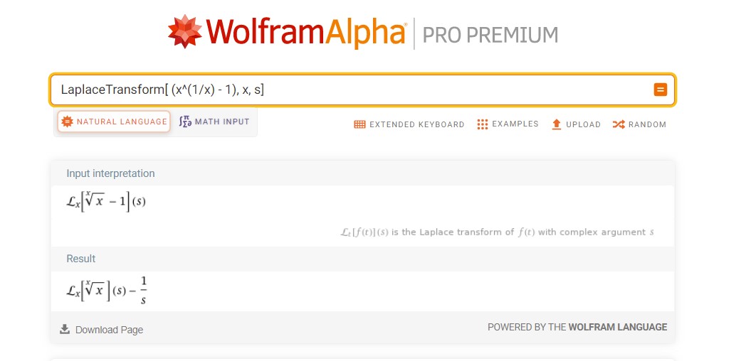
The Laplace transform analogy to the CMRB
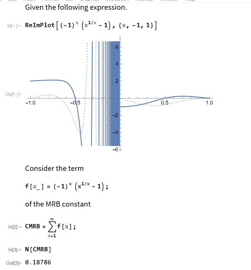
 see notebook
Likewise, Wolfram Alpha here says
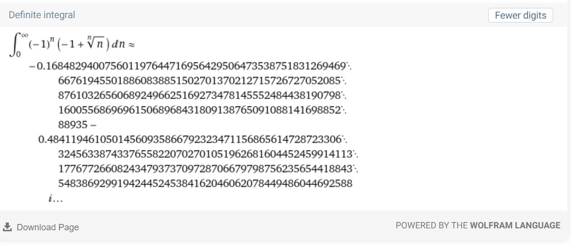
It also adds
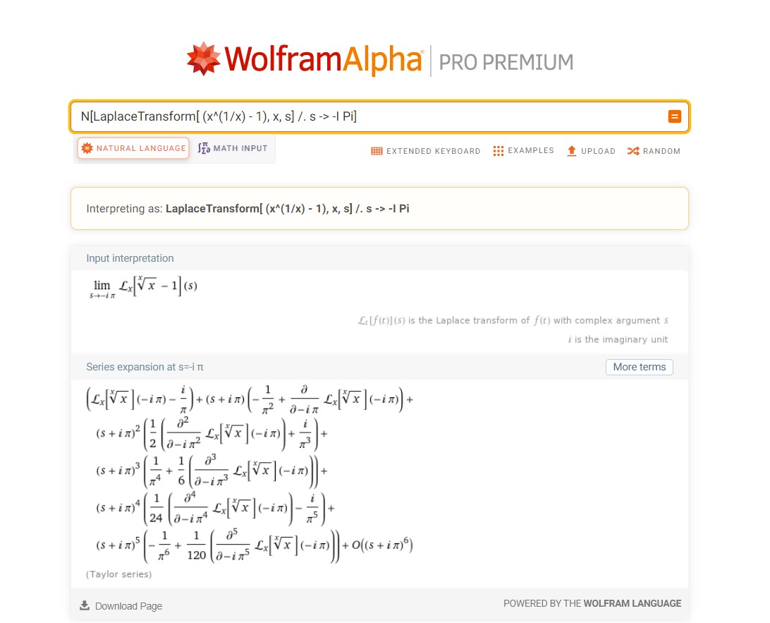
Interestingly,
That has the same argument,  , as the MeijerG transformation of CMRB.
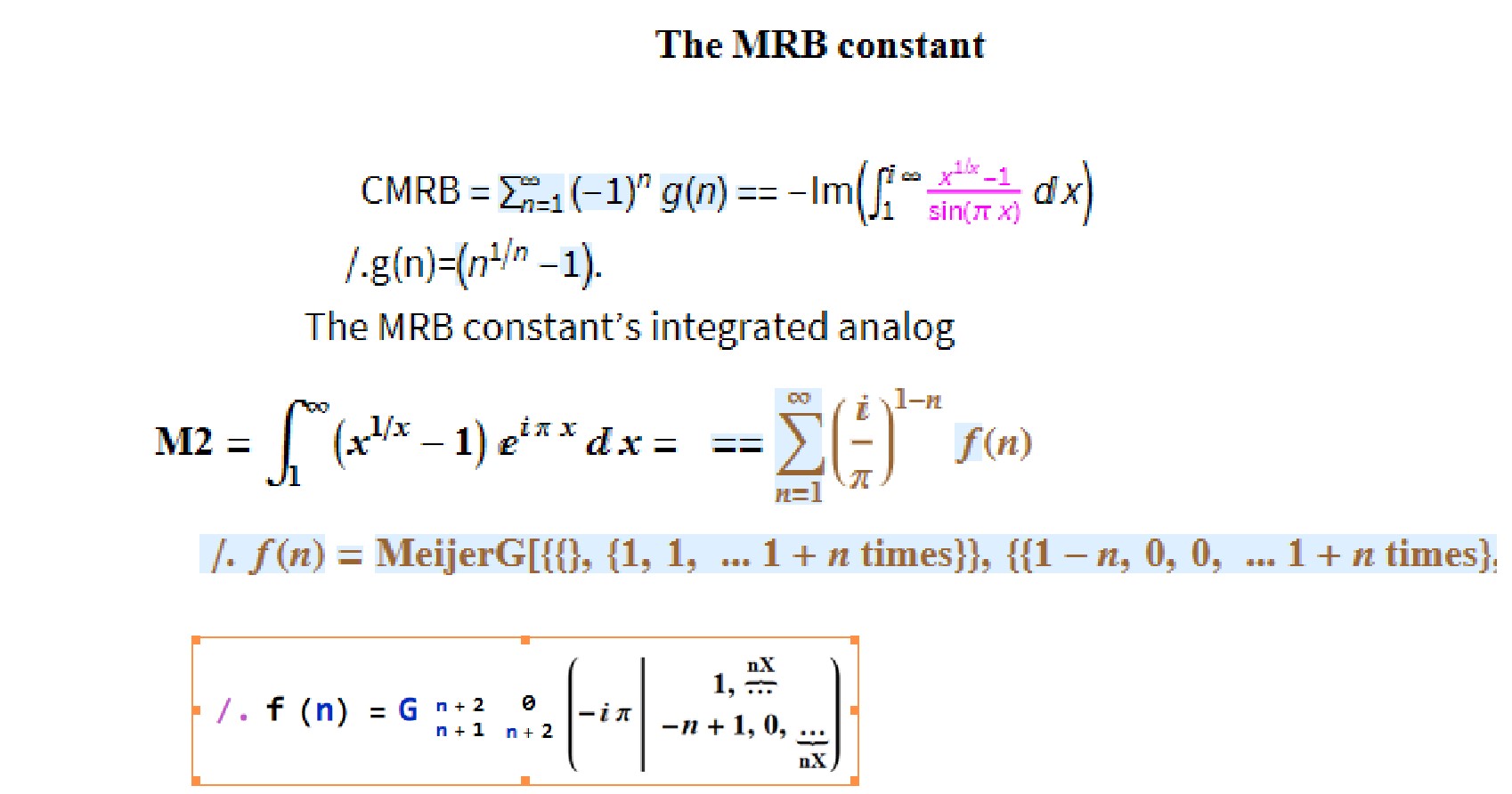
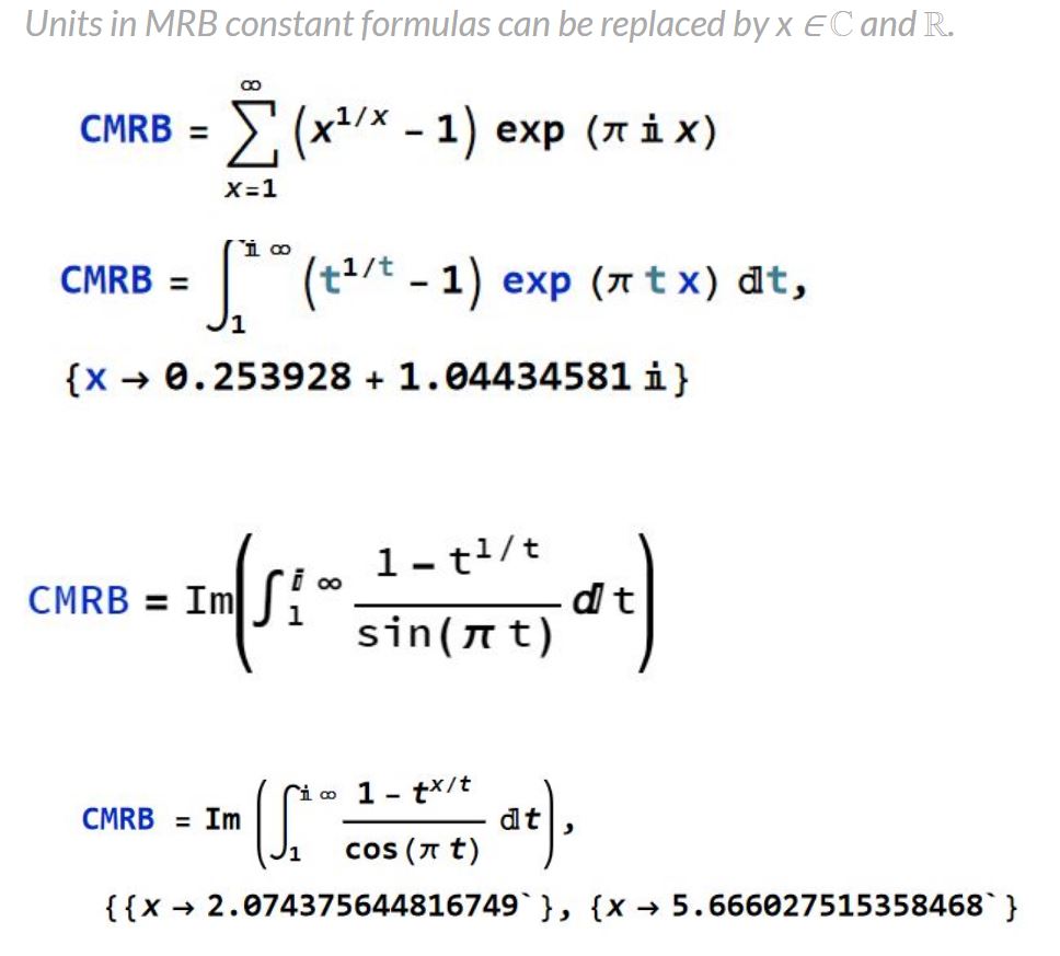
MRB constant formulas and identities
I developed this informal catalog of formulas for the MRB constant with over 20 years of research and ideas from users like you.
6/7/2022
CMRB
=
=
=
=
=
=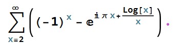
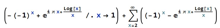
So, using induction, we have. 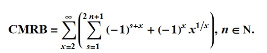
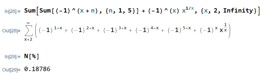
Sum[Sum[(-1)^(x + n), {n, 1, 5}] + (-1)^(x) x^(1/x), {x, 2, Infinity}]
3/25/2022
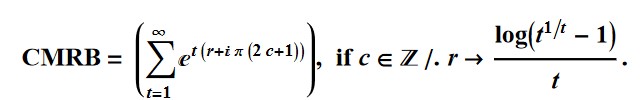
Formula (11) =
As Matheamatica says:
Assuming[Element[c, \[DoubleStruckCapitalZ]], FullSimplify[
     E^(t*(r + I*Pi*(2*c + 1))) /. r -> Log[t^(1/t) - 1]/t]]
= E^(I (1 + 2 c) [Pi] t) (-1 + t^(1/t)) 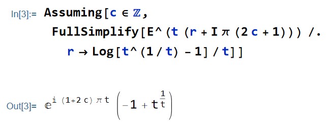
Where for all integers c, (1+2c) is odd leading to 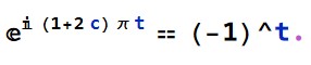
Expanding the E^log term gives
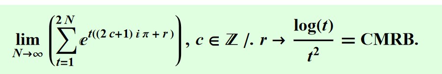
which is 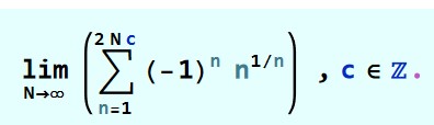 ,
,
That is exactly (2) in the above-quoted MathWorld definition: 
2/21/2022
Directly from the formula of 12/29/2021 below,  In
In
u = (-1)^t; N[
NSum[(t^(1/t) - 1) u, {t, 1, Infinity }, WorkingPrecision -> 24,
Method -> "AlternatingSigns"], 15]
Out[276]= 0.187859642462067
In
v = (-1)^-t - (-1)^t; 2 I N[
NIntegrate[Im[(t^(1/t) - 1) v^-1], {t, 1, Infinity I},
WorkingPrecision -> 24], 15]
Out[278]= 0.187859642462067
Likewise, 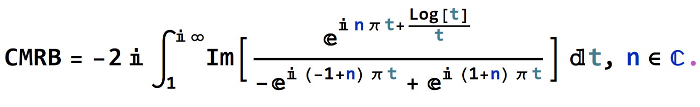
Expanding the exponents,
 This can be generalized to
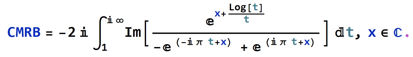
Building upon that, we get a closed form for the inner integral in the following.
CMRB= 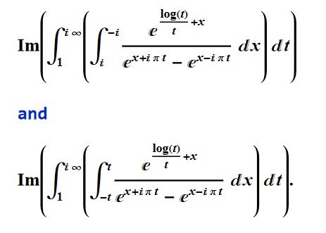
In[1]:=
CMRB = NSum[(-1)^n (n^(1/n) - 1), {n, 1, Infinity},
   WorkingPrecision -> 1000, Method -> "AlternatingSigns"];

In[2]:= CMRB - {
 Quiet[Im[NIntegrate[
    Integrate[
     E^(Log[t]/t + x)/(-E^((-I)*Pi*t + x) + E^(I*Pi*t + x)), {x,
      I, -I}], {t, 1, Infinity I}, WorkingPrecision -> 200,
    Method -> "Trapezoidal"]]];
 Quiet[Im[NIntegrate[
    Integrate[
     Im[E^(Log[t]/t + x)/(-E^((-I)*Pi*t + x) + E^(I*Pi*t + x))], {x,
      -t,  t }], {t, 1
     , Infinity  I}, WorkingPrecision -> 2000,
    Method -> "Trapezoidal"]]]}

Out[2]= {3.*10^-998, 3.*10^-998}
Which after a little analysis, can be shown convergent in the continuum limit at t → ∞ i.
12/29/2021
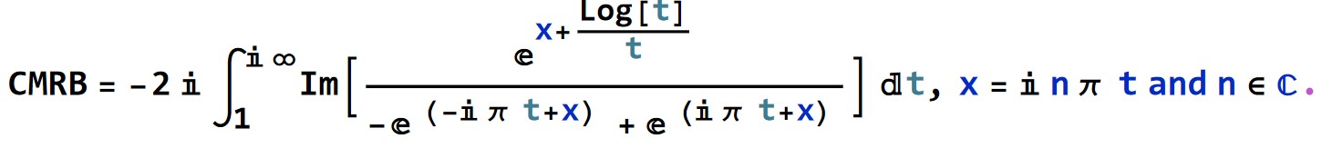
From "Primary Proof 1" worked below, it can be shown that 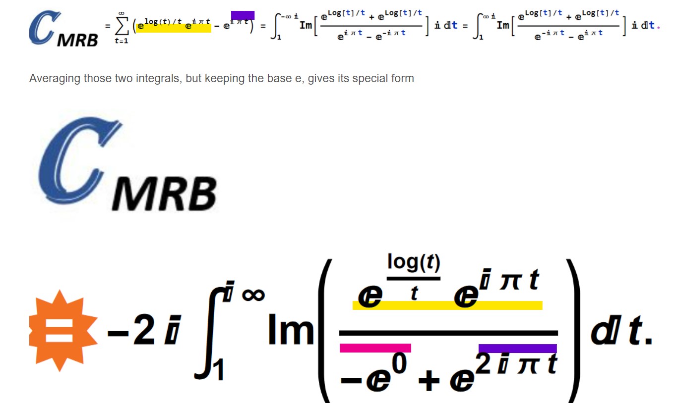
Mathematica knows that because
  m = N[NSum[-E^(I*Pi*t) + E^(I*Pi*t)*t^t^(-1), {t, 1, Infinity},
      Method -> "AlternatingSigns", WorkingPrecision -> 27], 18];
  Print[{m -
     N[NIntegrate[
       Im[(E^(Log[t]/t) + E^(Log[t]/t))/(E^(I \[Pi] t) -
            E^(-I \[Pi] t))] I, {t, 1, -Infinity I},
       WorkingPrecision -> 20], 18],
    m - N[NIntegrate[
       Im[(E^(Log[t]/t) + E^(Log[t]/t))/(E^(-I \[Pi] t) -
            E^(I \[Pi] t))] I, {t, 1, Infinity I},
       WorkingPrecision -> 20], 18],
    m + 2 I*NIntegrate[
       Im[(E^(I*Pi*t + Log[t]/t))/(-1 + E^((2*I)*Pi*t))], {t, 1,
        Infinity I}, WorkingPrecision -> 20]}]
yields
{0.*^-19,0.*^-19,0.*^-19}
Partial sums to an upper limit of (10^n i) give approximations for the MRB constant + the same approximation *10^-(n+1) i. Example:
-2 I*NIntegrate[
  Im[(E^(I*Pi*t + Log[t]/t))/(-1 + E^((2*I)*Pi*t))], {t, 1, 10^7 I},
  WorkingPrecision -> 20]
gives 0.18785602000738908694 + 1.878560200074*10^-8 I where CMRB ≈ 0.187856.
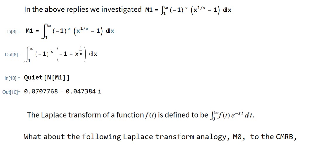
Notice it is special because if we integrate only the numerator, we have MKB=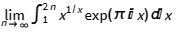 , which defines the "integrated analog of CMRB" (MKB) described by Richard Mathar in https://arxiv.org/abs/0912.3844. (He called it M1.)
Like how this:
NIntegrate[(E^(I*Pi*t + Log[t]/t)), {t, 1, Infinity I},
  WorkingPrecision -> 20] - I/Pi
converges to
0.070776039311528802981 - 0.68400038943793212890 I.
(The upper limits " i infinity" and " infinity" produce the same result in this integral.)
11/14/2021
Here is a standard notation for the above mentioned
CMRB,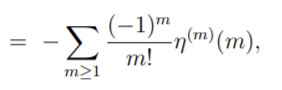
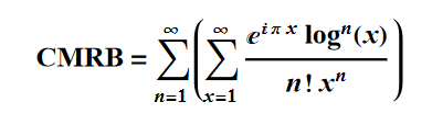 .
.
In[16]:= CMRB = 0.18785964246206712024851793405427323005590332204; \
CMRB - NSum[(Sum[
    E^(I \[Pi] x) Log[x]^n/(n! x^n), {x, 1, Infinity}]), {n, 1, 20},
  WorkingPrecision -> 50]

Out[16]= -5.8542798212228838*10^-30

In[8]:= c1 =
 Activate[Limit[(-1)^m/m! Derivative[m][DirichletEta][x] /. m -> 1,
   x -> 1]]

Out[8]= 1/2 Log[2] (-2 EulerGamma + Log[2])

In[14]:= CMRB -
 N[-(c1 + Sum[(-1)^m/m! Derivative[m][DirichletEta][m], {m, 2, 20}]),
  30]

Out[14]= -6.*10^-30
11/01/2021
: The catalog now appears complete, and can all be proven through Primary Proof 1, and the one with the eta function, Primary Proof 2, both found below.
a ≠b 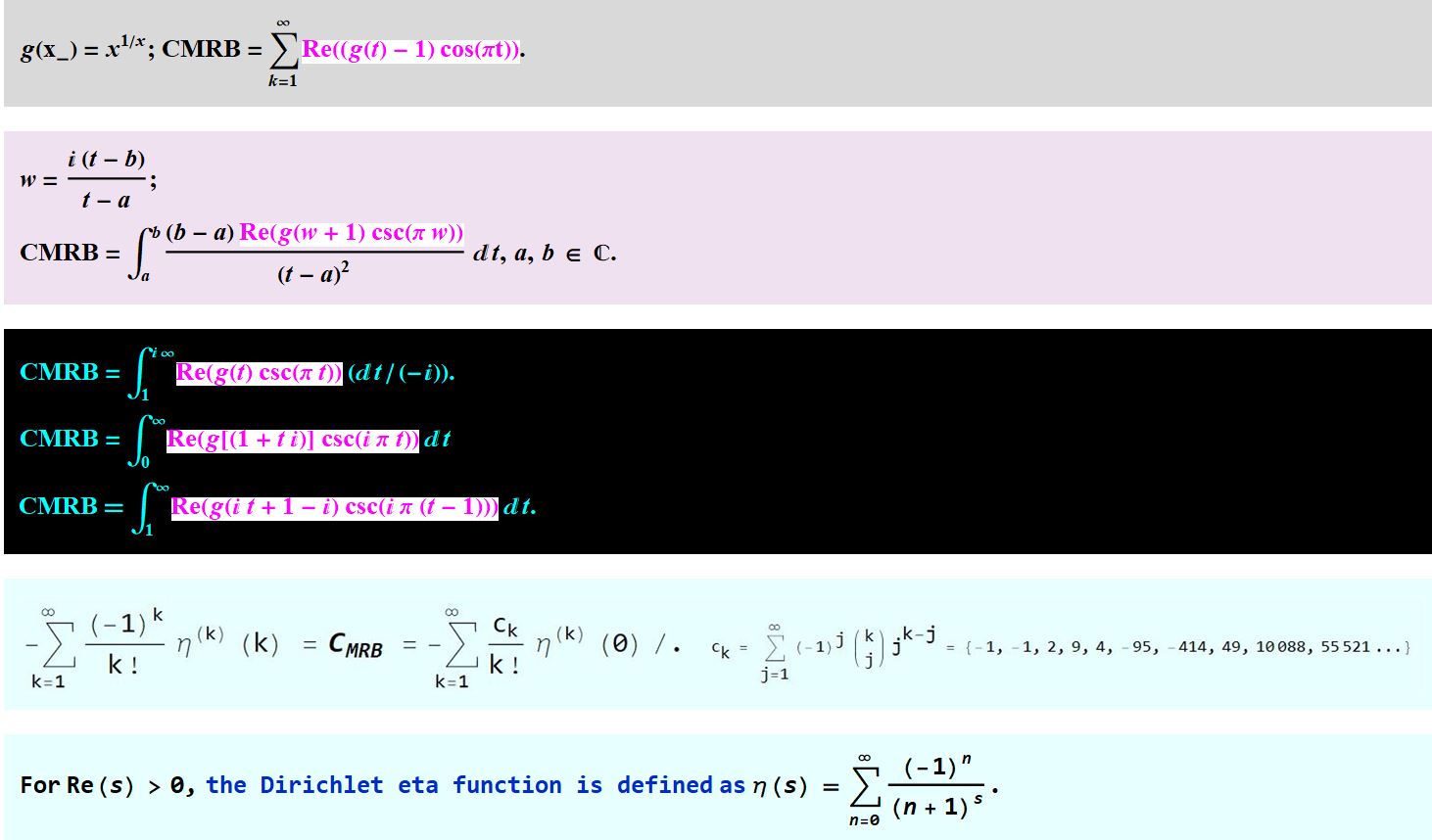
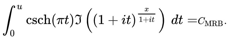
g[x_] = x^(1/x); CMRB =
NSum[(-1)^k (g[k] - 1), {k, 1, Infinity}, WorkingPrecision -> 100,
Method -> "AlternatingSigns"]; a = -Infinity I; b = Infinity I;
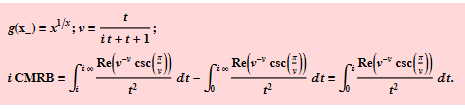
g[x_] = x^(1/x); (v = t/(1 + t + t I);
Print[CMRB - (-I /2 NIntegrate[ Re[v^-v Csc[Pi/v]]/ (t^2), {t, a, b},
WorkingPrecision -> 100])]); Clear[a, b]
-9.3472*10^-94
Thus, we find
here, and  next:
next:
In[93]:= CMRB =
 NSum[Cos[Pi n] (n^(1/n) - 1), {n, 1, Infinity},
  Method -> "AlternatingSigns", WorkingPrecision -> 100]; Table[
 CMRB - (1/2 +
    NIntegrate[
     Im[(t^(1/t) - t^(2 n))] (-Csc[\[Pi] t]), {t, 1, Infinity I},
     WorkingPrecision -> 100, Method -> "Trapezoidal"]), {n, 1, 5}]

Out[93]= {-9.3472*10^-94, -9.3473*10^-94, -9.3474*10^-94, \
-9.3476*10^-94, -9.3477*10^-94}
CNT+F "The following is a way to compute the" for more evidence
For such n, 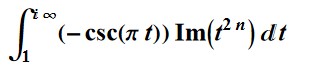 converges to 1/2+0i.
(How I came across all of those and more example code follow in various replies.)
On 10/18/2021
, I found the following triad of pairs of integrals summed from -complex infinity to +complex infinity.
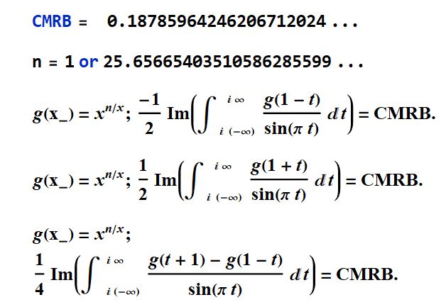
You can see it worked in this link here.
In[1]:= n = {1, 25.6566540351058628559907};

In[2]:= g[x_] = x^(n/x);
-1/2 Im[N[
   NIntegrate[(g[(1 - t)])/(Sin[\[Pi] t]), {t, -Infinity I,
     Infinity I}, WorkingPrecision -> 60], 20]]

Out[3]= {0.18785964246206712025, 0.18785964246206712025}

In[4]:= g[x_] = x^(n/x);
1/2 Im[N[NIntegrate[(g[(1 + t)])/(Sin[\[Pi] t]), {t, -Infinity I,
     Infinity I}, WorkingPrecision -> 60], 20]]

Out[5]= {0.18785964246206712025, 0.18785964246206712025}

In[6]:= g[x_] = x^(n/x);
1/4 Im[N[NIntegrate[(g[(1 + t)] - (g[(1 - t)]))/(Sin[\[Pi] t]), {t, -Infinity I,
     Infinity I}, WorkingPrecision -> 60], 20]]

Out[7]= {0.18785964246206712025, 0.18785964246206712025}
Therefore, bringing
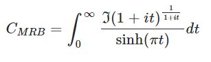
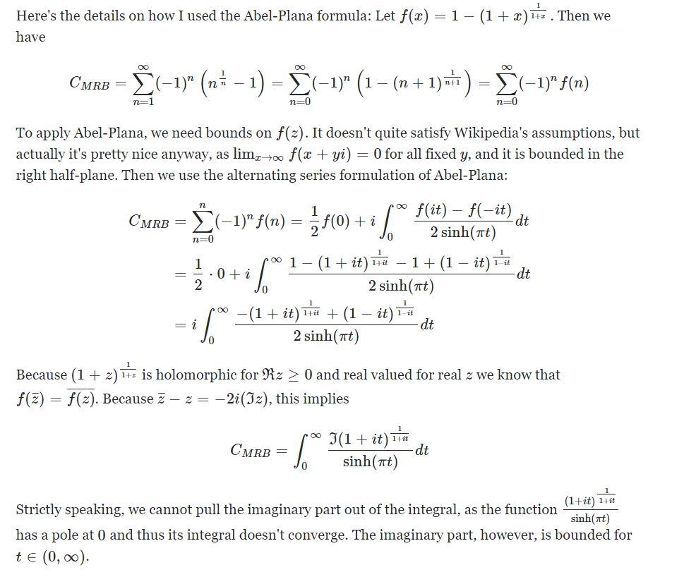
back to mind, we joyfully find,
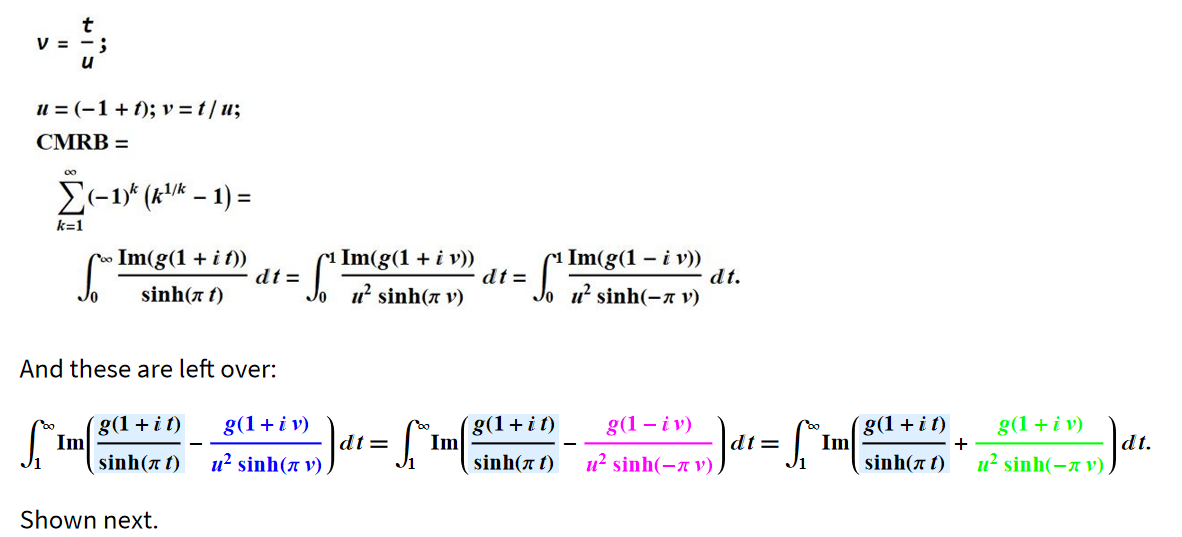
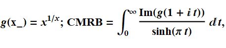
In[1]:= n =
  25.65665403510586285599072933607445153794770546058072048626118194900\
97321718621288009944007124739159792146480733342667`100.;

g[x_] = {x^(1/x), x^(n/x)};

CMRB = NSum[(-1)^k (k^(1/k) - 1), {k, 1, Infinity},
   WorkingPrecision -> 100, Method -> "AlternatingSigns"];

Print[CMRB -
  NIntegrate[Im[g[(1 + I t)]/Sinh[\[Pi] t]], {t, 0, Infinity},
   WorkingPrecision -> 100], u = (-1 + t); v = t/u;
 CMRB - NIntegrate[Im[g[(1 + I v)]/(Sinh[\[Pi] v] u^2)], {t, 0, 1},
   WorkingPrecision -> 100],
 CMRB - NIntegrate[Im[g[(1 - I v)]/(Sinh[-\[Pi] v] u^2)], {t, 0, 1},
   WorkingPrecision -> 100]]

During evaluation of In[1]:= {-9.3472*10^-94,-9.3472*10^-94}{-9.3472*10^-94,-9.3472*10^-94}{-9.3472*10^-94,-9.3472*10^-94}

In[23]:= Quiet[
 NIntegrate[
  Im[g[(1 + I t)]/Sinh[\[Pi] t] -
    g[(1 + I v)]/(Sinh[\[Pi] v] u^2)], {t, 1, Infinity},
  WorkingPrecision -> 100]]

Out[23]= -3.\
9317890831820506378791034479406121284684487483182042179057328100219696\
20202464096600592983999731376*10^-55

In[21]:= Quiet[
 NIntegrate[
  Im[g[(1 + I t)]/Sinh[\[Pi] t] -
    g[(1 - I v)]/(Sinh[-\[Pi] v] u^2)], {t, 1, Infinity},
  WorkingPrecision -> 100]]

Out[21]= -3.\
9317890831820506378791034479406121284684487483182042179057381396998279\
83065832972052160228141179706*10^-55

In[25]:= Quiet[
 NIntegrate[
  Im[g[(1 + I t)]/Sinh[\[Pi] t] +
    g[(1 + I v)]/(Sinh[-\[Pi] v] u^2)], {t, 1, Infinity},
  WorkingPrecision -> 100]]

Out[25]= -3.\
9317890831820506378791034479406121284684487483182042179057328100219696\
20202464096600592983999731376*10^-55
On 9/29/2021
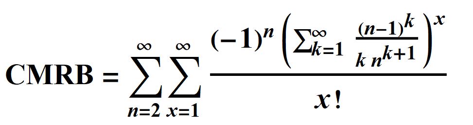
I found the following equation for CMRB (great for integer arithmetic because
(1-1/n)^k=(n-1)^k/n^k. )
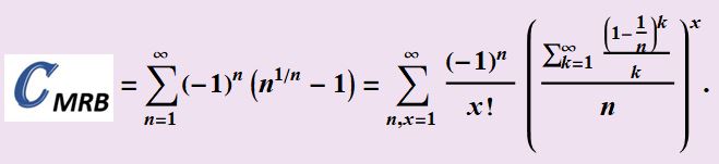
So, using only integers, and sufficiently large ones in place of infinity, we can use
See
In[1]:= Timing[m=NSum[(-1)^n (n^(1/n)-1),{n,1,Infinity},WorkingPrecision->200,Method->"AlternatingSigns"]][[1]]

Out[1]= 0.086374

In[2]:= Timing[m-NSum[(-1)^n/x! (Sum[((-1 + n)^k) /(k n^(1 + k)), {k, 1, Infinity}])^ x, {n, 2, Infinity}, {x, 1,100}, Method -> "AlternatingSigns",  WorkingPrecision -> 200, NSumTerms -> 100]]

Out[2]= {17.8915,-2.2*^-197}
It is very much slower, but it can give a rational approximation (p/q), like in the following.
In[3]:= mt=Sum[(-1)^n/x! (Sum[((-1 + n)^k) /(k n^(1 + k)), {k, 1,500}])^ x, {n, 2,500}, {x, 6}];

In[4]:= N[m-mt]

Out[4]= -0.00602661

In[5]:= Head[mt]

Out[5]= Rational
Compared to the NSum formula for m, we see
In[6]:= Head[m]

Out[6]= Real
On 9/19/2021
I found the following quality of CMRB.
On 9/5/2021
I added the following MRB constant integral over an unusual range.
See proof in this link here.
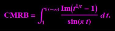
On Pi Day, 2021, 2:40 pm EST,
I added a new MRB constant integral.


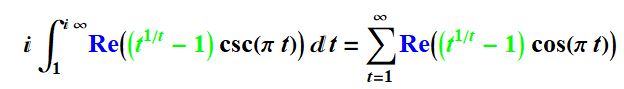
We see many more integrals for CMRB.
We can expand 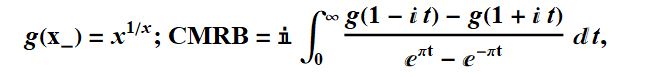 into the following.

xx = 25.65665403510586285599072933607445153794770546058072048626118194\
90097321718621288009944007124739159792146480733342667`100.;


g[x_] = x^(xx/
    x); I NIntegrate[(g[(-t I + 1)] - g[(t I + 1)])/(Exp[Pi t] -
           Exp[-Pi t]), {t, 0, Infinity}, WorkingPrecision -> 100]

 (*
0.18785964246206712024851793405427323005590309490013878617200468408947\
72315646602137032966544331074969.*)
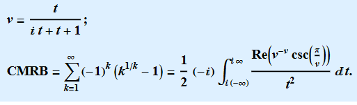
Expanding upon the previously mentioned
we get the following set of formulas that all equal CMRB:
Let
x= 25.656654035105862855990729 ...
along with the following constants (approximate values given)
{u = -3.20528124009334715662802858},
{u = -1.975955817063408761652299},
{u = -1.028853359952178482391753},
{u = 0.0233205964164237996087020},
{u = 1.0288510656792879404912390},
{u = 1.9759300365560440110320579},
{u = 3.3776887945654916860102506},
{u = 4.2186640662797203304551583} or
$ u = \infty .$
Another set follows.
let x = 1 and
along with the following {approximations}
{u = 2.451894470180356539050514},
{u = 1.333754341654332447320456} or
$ u = \infty $
then
See this notebook from the wolfram cloud for justification.
2020 and before:
Also, in terms of the Euler-Riemann zeta function,
CMRB =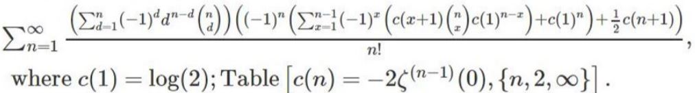
Furthermore, as 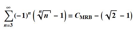 ,
,
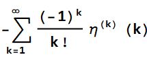
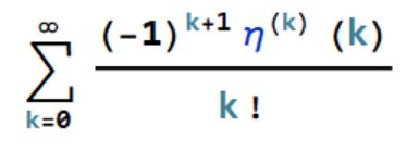
according to user90369 at Stack Exchange, CMRB can be written as the sum of zeta derivatives similar to the eta derivatives discovered by Crandall.  Information about η(j)(k) please see e.g. this link here, formulas (11)+(16)+(19).
In the light of the parts above, where
CMRB
= 
= 
= 
 as well as
 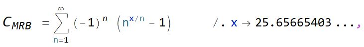 an internet scholar going by the moniker "Dark Malthorp" wrote:
Primary Proof 1
CMRB= , based on
CMRB 
is proven below by an internet scholar going by the moniker "Dark Malthorp."
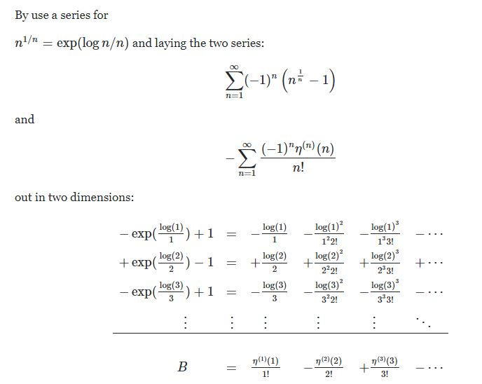
Primary Proof 2
 denoting the kth derivative of the Dirichlet eta function of k and 0 respectively, was first discovered in 2012 by Richard Crandall of Apple Computer.
The left half is proven below by Gottfried Helms and it is proven more rigorously considering the conditionally convergent sum,
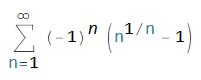
 below that. Then the right half is a Taylor expansion of eta(s) around s = 0.
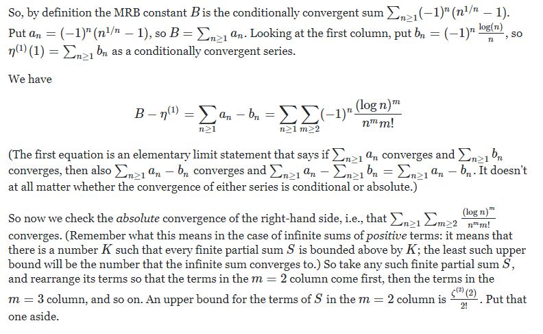
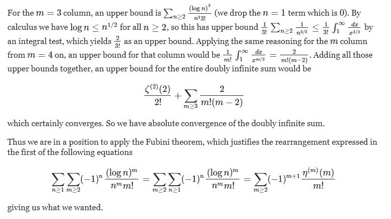
At https://math.stackexchange.com/questions/1673886/is-there-a-more-rigorous-way-to-show-these-two-sums-are-exactly-equal,
it has been noted that "even though one has cause to be a little bit wary around formal rearrangements of conditionally convergent sums (see the Riemann series theorem), it's not very difficult to validate the formal manipulation of Helms. The idea is to cordon off a big chunk of the infinite double summation (all the terms from the second column on) that we know is absolutely convergent, which we are then free to rearrange with impunity. (Most relevantly for our purposes here, see pages 80-85 of this document, culminating with the Fubini theorem which is essentially the manipulation Helms is using.)"
Primary Proof 3
Here is proof of a faster converging integral for its integrated analog (The MKB constant) by Ariel Gershon.
g(x)=x^(1/x), M1=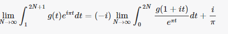
Which is the same as
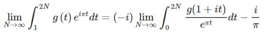 because changing the upper limit to 2N + 1 increases MI by 2i/?.
MKB constant calculations have been moved to their discussion at http://community.wolfram.com/groups/-/m/t/1323951?ppauth=W3TxvEwH .
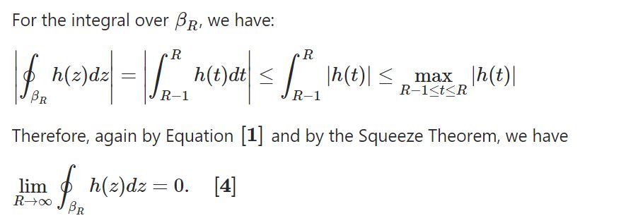
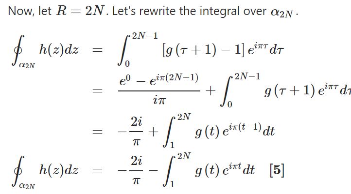
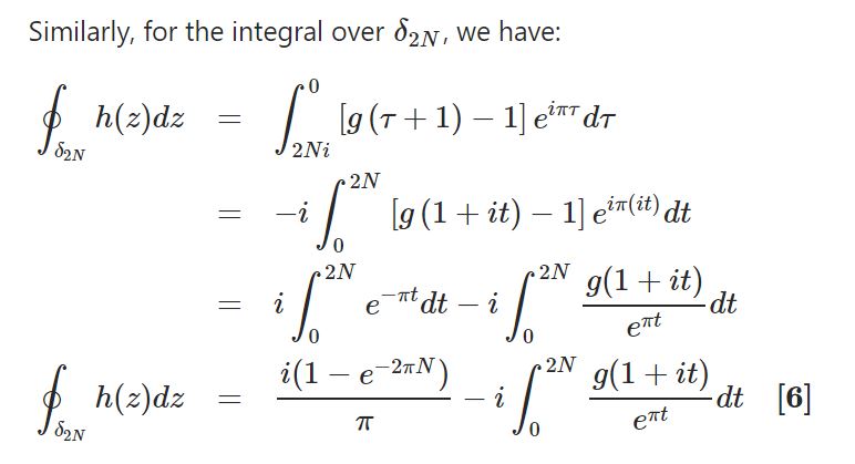
Plugging in equations [5] and [6] into equation [2] gives us:
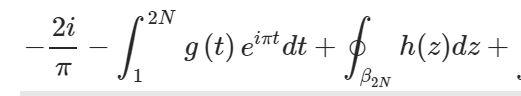
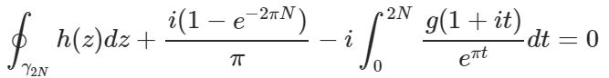
Now take the limit as N?? and apply equations [3] and [4] : 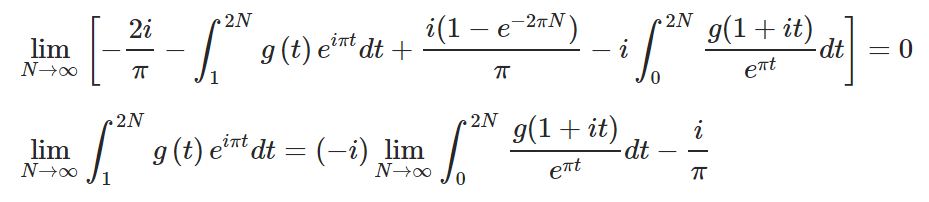 He went on to note that
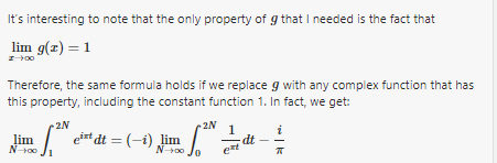
I wondered about the relationship between CMRB and its integrated analog and asked the following. 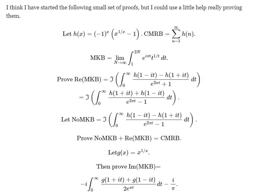 So far I came up with
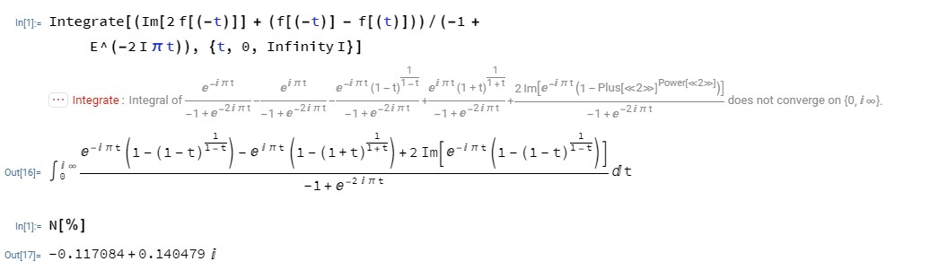
Another relationship between the sum and integral that remains more unproven than I would like is
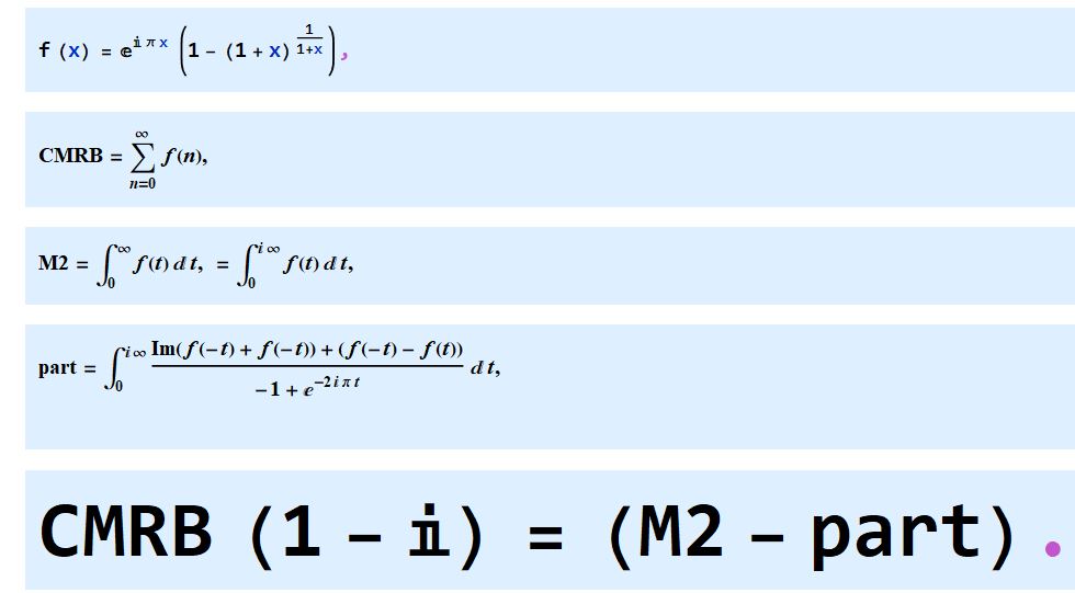
f[x_] = E^(I \[Pi] x) (1 - (1 + x)^(1/(1 + x)));
CMRB = NSum[f[n], {n, 0, Infinity}, WorkingPrecision -> 30,
   Method -> "AlternatingSigns"];
M2 = NIntegrate[f[t], {t, 0, Infinity I}, WorkingPrecision -> 50];
part = NIntegrate[(Im[2 f[(-t)]] + (f[(-t)] - f[(t)]))/(-1 +
      E^(-2 I \[Pi] t)), {t, 0, Infinity I}, WorkingPrecision -> 50];
CMRB (1 - I) - (M2 - part)
gives
6.10377910^-23 - 6.10377910^-23 I.
Where the integral does not converge, but Mathematica can give it a value:
Update 2015
Here is my mini-cluster of the fastest 3 computers (the MRB constant supercomputer 0) mentioned below: The one to the left is my custom-built extreme edition 6 core and later with an 8 core 3.4 GHz Xeon processor with 64 GB 1666 MHz RAM.. The one in the center is my fast little 4-core Asus with 2400 MHz RAM. Then the one on the right is my fastest -- a Digital Storm 6 core overclocked to 4.7 GHz on all cores and with 3000 MHz RAM.

see notebook
Likewise, Wolfram Alpha here says
It also adds
Interestingly,
That has the same argument, , as the MeijerG transformation of CMRB.


