In recent explorations how to generate randomness from physical systems consisting of massive disks bouncing around according to typical conservation laws, we've encountered difficult corner cases quite unlike the usual low density limit. The purpose of this memo is to answer two questions: What happens to typical high-school collision formula when two or more collisions happen simultaneously? Can a consistent solution be found by modifying the usual equations?
Assuming that we already know what happens in a two-body elastic collision, let's start with the simplest examples of a simultaneous three-body collision, such as follows:
vel = {
   {v1 Cos[\[Theta]1 - \[Delta]1], v1 Sin[\[Theta]1 - \[Delta]1]},
   {v2 Cos[\[Theta]2 - \[Delta]2], v2 Sin[\[Theta]2 - \[Delta]2]},
   {0, 0}
   };

pos = {
   { -Cos[\[Theta]1 ], -Sin[\[Theta]1]},
   { -Cos[\[Theta]2 ], -Sin[\[Theta]2]},
   {0, 0}
   };

Grid[Partition[Table[
   With[{randomCollision = {
       m1 -> 1, m2 -> 1, ms -> 1,
       \[Theta]1 -> 0,
       \[Theta]2 -> -RandomReal[{Pi/3, Pi}],
       \[Delta]1 -> 0,
       \[Delta]2 -> 0,
       v1 -> 1, v2 -> 1}},
    Graphics[MapThread[{White, EdgeForm[Black],
        Disk[#1, 1/2],
        Gray, Arrow[{#1 - #2, #1}]
        } &, {pos /. randomCollision, vel /. randomCollision}],
     PlotRange -> {{-2, 2}, {-1, 2}}
     ]], {12}], 3]]
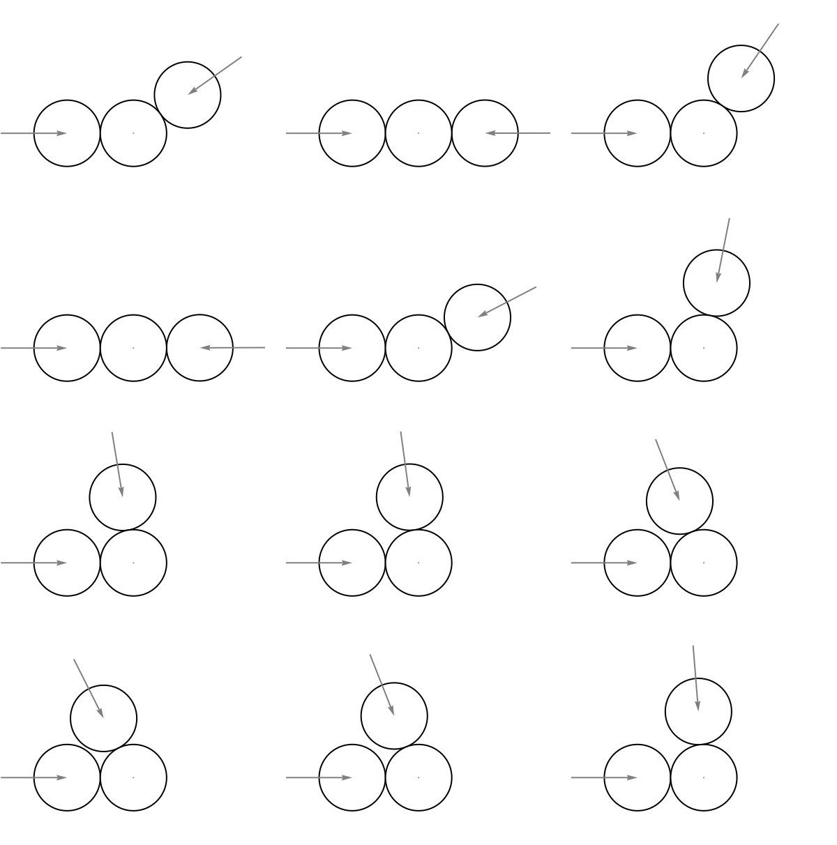
A frame of reference has been chosen with the center mass fixed. The impinging masses have equal velocities, which are both directed toward the centroid of the fixed mass. A common first idea is: "Well, what if applying collisions in sequence doesn't produce a noticeable difference?" It's a bit hopeful, though, not entirely wrong. We test this idea by defining a commutator for order of operations as follows:
MomentumDifferential[dx_, v1In_, v2In_, m1In_, m2In_
  ] := Times[Divide[2 m1In*m2In, m1In + m2In],
  Dot[v1In - v2In, dx]*dx]

TwoPartCollisionSymmetryBroken[{dx1_, v1In_}, {dx2_, v2In_}
  ] := Module[{dp1s, dp2s, mag, v1Out, v2Out, vsOut},
  dp1s = MomentumDifferential[dx1, v1In, {0, 0}, m1, ms];
  dp2s = MomentumDifferential[dx2, v2In, dp1s/ms, m2, ms];
  v1Out = v1In - dp1s/m1;
  v2Out = v2In - dp2s/m2;
  vsOut = dp1s/ms + dp2s/ms;
  {v1Out, v2Out, vsOut}
  ]

v1Solution = TwoPartCollisionSymmetryBroken[{
    { -Cos[\[Theta]1 ], -Sin[\[Theta]1]},
    {v1 Cos[\[Theta]1 - \[Delta]1], v1 Sin[\[Theta]1 - \[Delta]1]}
    }, {
    { -Cos[\[Theta]2 ], -Sin[\[Theta]2]},
    {v2 Cos[\[Theta]2 - \[Delta]2], v2 Sin[\[Theta]2 - \[Delta]2]}
    }];

v2Solution = TwoPartCollisionSymmetryBroken[{
     { -Cos[\[Theta]2 ], -Sin[\[Theta]2]},
     {v2 Cos[\[Theta]2 - \[Delta]2], v2 Sin[\[Theta]2 - \[Delta]2]}
     }, {
     { -Cos[\[Theta]1 ], -Sin[\[Theta]1]},
     {v1 Cos[\[Theta]1 - \[Delta]1], v1 Sin[\[Theta]1 - \[Delta]1]}
     }][[{2, 1, 3}]];

commutator = ReplaceAll[Refine[Sqrt[Simplify@ReplaceAll[
      # . # & /@ (v1Solution - v2Solution),
      {m1 -> 1, m2 -> 1, ms -> 1, \[Delta]1 -> 0, \[Delta]2 -> 0,
       \[Theta]1 -> \[Theta] + \[Theta]2, v1 -> 1,
       v2 -> 1}]], \[Theta] \[Element] Reals],
  Abs -> Identity]

Out[] = {Cos[\[Theta]], Cos[\[Theta]], 2 Cos[\[Theta]] Sin[\[Theta]/2]}

Plot[commutator, {\[Theta], 0, 2 Pi}, PlotRange -> All]
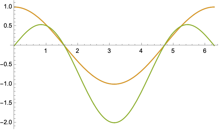
The resulting commutators for each output velocity vector, $\{\cos[\theta], \cos[\theta], 2\cos[\theta] \sin[\theta/2 \}$, have all zeroes at $\theta = \pm \pi/2$ where the input velocity vectors decompose along orthogonal dimensions. Otherwise there is generally a difference when colliding one particle first and the other second (as compared to the vice versa colliding the other first and the one second). To get a visual sense of this, we can plot alternative output vectors in Red and Blue:
With[{simpleCollision = {m1 -> 1, m2 -> 1,
    ms -> 1, \[Delta]1 -> 0, \[Delta]2 -> 0, v1 -> 1, v2 -> 1}},
 With[{
   vAsym1 =
    Expand[v1Solution /.
       simpleCollision /. {\[Theta]1 -> -Pi/5, \[Theta]2 -> Pi/5}],
   vAsym2 =
    Expand[v2Solution /.
       simpleCollision /. {\[Theta]1 -> -Pi/5, \[Theta]2 -> Pi/5}]
   },
  Graphics[MapThread[{White, EdgeForm[Black], Disk[#1, 1/2],
      Red, Arrow[{#1, #1 + #2}],
      Blue, Arrow[{#1, #1 + #3}]
      } &, {pos /.
       simpleCollision /. {\[Theta]1 -> -Pi/5, \[Theta]2 -> Pi/5},
     vAsym1, vAsym2}]]
  ]]
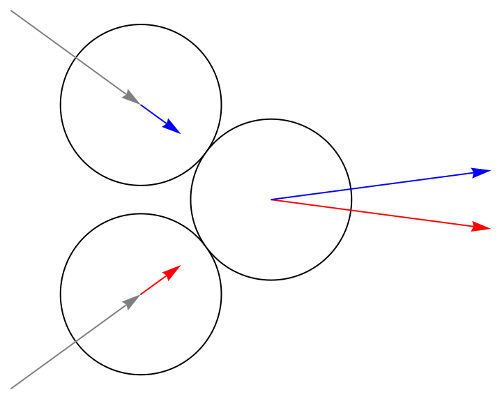
Of course, whichever collision happens first completely stops one disk, and then subsequently reduces the velocity of the other. Considering symmetry, this doesn't seem right at all, and we don't already have a way to continuously vary between solutions to find the mean we're looking for. What can we do?
Let's assume that disks exchange momenta in increments $\pm dp_{1s}$ and $\pm dp_{2s}$ with $s$ standing for "initially still". The output momenta can then be written as: $$p_1 ' = p_1 - k\cdot dp_{1s},$$ $$p_2 ' = p_2 - k\cdot dp_{2s}, $$ $$p_s ' = k\cdot( dp_{1s}+dp_{2s}). $$
Where the constant $k$ can be determined from conservation of energy. By design the sum of momenta is conservative, and because the differentials point toward or away from the center of the still disk, their addition also conserves angular momentum. So this is a valid solution with regard to fundamental principles, but also one where an arbitrary scaling choice has been made.
TwoPartCollisionSymmetric[{dx1_, v1In_}, {dx2_, v2In_}
  ] := Module[{
   dp1s = scale*MomentumDifferential[dx1, v1In, {0, 0}, m1, ms],
   dp2s = scale*MomentumDifferential[dx2, v2In, {0, 0}, m2, ms],
   mag, v1Out, v2Out, vsOut},
  v1Out = v1In - dp1s/m1;
  v2Out = v2In - dp2s/m2;
  vsOut = dp1s/ms + dp2s/ms;
  mag = First[DeleteCases[
     scale /.
       Solve[Simplify@Subtract[m1 v1In . v1In + m2 v2In . v2In,
           Dot[Dot[#, #] & /@ {m1 v1Out, m2 v2Out, ms vsOut},
            {1/m1, 1/m2, 1/ms}]] == 0, scale
        ] /. Abs -> Identity, 0]];
  {v1Out, v2Out, vsOut} /. {
    scale -> mag, Abs -> Identity
    }]

genVecs1 = Simplify@Expand[
    TwoPartCollisionSymmetric[{
      { -Cos[\[Theta]1 ], -Sin[\[Theta]1]},
      {v1 Cos[\[Theta]1 - \[Delta]1], v1 Sin[\[Theta]1 - \[Delta]1]}
      }, {
      { -Cos[\[Theta]2 ], -Sin[\[Theta]2]},
      {v2 Cos[\[Theta]2 - \[Delta]2], v2 Sin[\[Theta]2 - \[Delta]2]}
      }]];
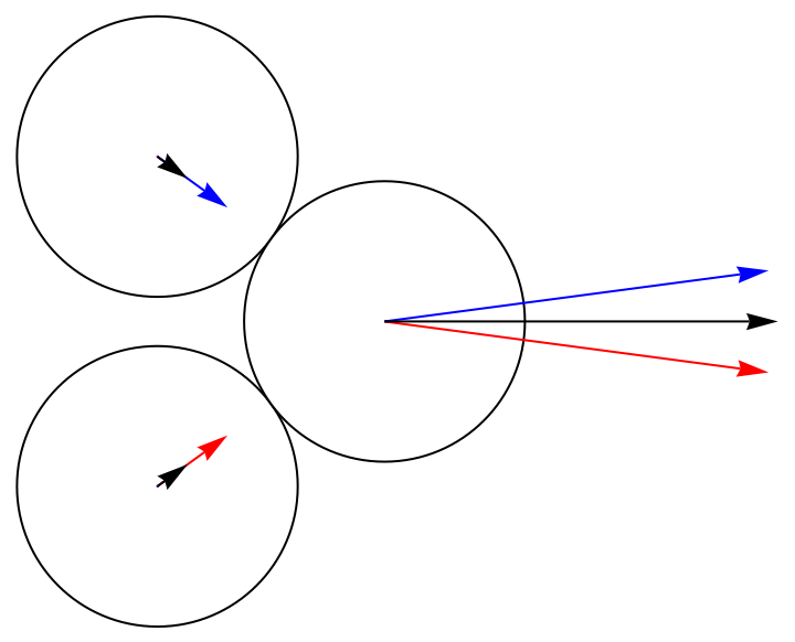
And we can see by updating the collision plot that this technique produces a much better result:
With[{simpleCollision = {m1 -> 1, m2 -> 1,
    ms -> 1, \[Delta]1 -> 0, \[Delta]2 -> 0, v1 -> 1, v2 -> 1}},
 With[{
   vAsym1 =
    Expand[v1Solution /.
       simpleCollision /. {\[Theta]1 -> -Pi/5, \[Theta]2 -> Pi/5}],
   vAsym2 =
    Expand[v2Solution /.
       simpleCollision /. {\[Theta]1 -> -Pi/5, \[Theta]2 -> Pi/5}],
   vSym =
    Expand[genVecs1 /.
       simpleCollision /. {\[Theta]1 -> -Pi/5, \[Theta]2 -> Pi/5}]
   },
  Graphics[MapThread[{White, EdgeForm[Black], Disk[#1, 1/2],
      Red, Arrow[{#1, #1 + #2}],
      Blue, Arrow[{#1, #1 + #3}],
      Black, Arrow[{#1, #1 + #4}]
      } &, {pos /.
       simpleCollision /. {\[Theta]1 -> -Pi/5, \[Theta]2 -> Pi/5},
     vAsym1, vAsym2, vSym}]]
  ]]
We also get seemingly acceptable results if we allow disks to collide with skew vectors:
GraphicsGrid@Partition[Table[With[{randomCollision = {
       m1 -> 1, m2 -> 1, ms -> 1,
       \[Theta]1 -> 0,
       \[Theta]2 -> -RandomReal[{Pi/3, Pi}],
       \[Delta]1 -> RandomReal[{-Pi/4, Pi/4}],
       \[Delta]2 -> RandomReal[{-Pi/4, Pi/4}], v1 -> 1, v2 -> 1}},
    With[{
      vAsym1 = Expand[v1Solution /. randomCollision],
      vAsym2 = Expand[v2Solution /. randomCollision],
      vSym = Expand[genVecs1 /. randomCollision]},
     Graphics[MapThread[{White, EdgeForm[Black],
         Disk[#1, 1/2],
         Gray, Arrow[{#1 - #2, #1}],
         Red, Arrow[{#1, #1 + #3}],
         Blue, Arrow[{#1, #1 + #4}],
         Black, Arrow[{#1, #1 + #5}]
         } &, {pos /. randomCollision, vel /. randomCollision,
        vAsym1, vAsym2, vSym}],
      PlotRange -> {{-2, 2}, {-1, 2}}
      ]]], {16}], 4]
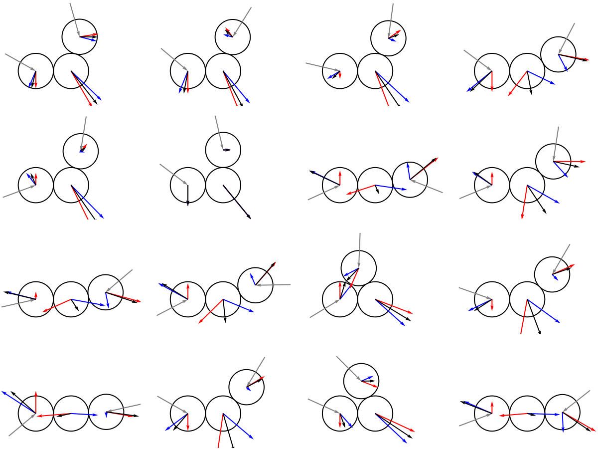
Unfortunately, if we try to add a fourth body, it quickly becomes easy to accidentally violate conservation of angular momentum. So more work remains to be done finding an acceptable, exactly solve-able, semi-realistic convention for dealing with corner cases of hard circle collision simulations.


